1. Introduction

Magnetic resonance imaging (MRI) is an imaging technique used primarily in medical settings to produce high quality images of the inside of the human body. MRI is based on the principles of nuclear magnetic resonance (NMR), a spectroscopic technique used by scientists to obtain microscopic chemical and physical information about molecules. The technique was called magnetic resonance imaging rather than nuclear magnetic resonance imaging (NMRI) because of the negative connotations associated with the word nuclear. [1]. Artifacts caused by head and body motion pose a significant problem for the in vivo magnetic resonance imaging (MRI) of the human brain. Motion artifacts adversely affect the ability to accurately characterize the size, shape, and tissue properties of brain structures in both research subjects and clinical patients. In cognitive neuroscience applications, cross-sectional and longitudinal effects in neuroanatomical measurements are relatively small, making them easily obscured by distortions arising from patient and subject movement. Image quality is often degraded by motion artifacts, including image blurring and ghosting [1]. A number of techniques are employed to help in get rid of these problems: one is to prevent the motion occurring using sedation or physical restraints. Sedation involves risk [2] and also adds complication to the scan. Physically restraining patients is only partially effective. The objectives of this Thesis first is to develop algorithm to correct the motion blur in the MRI image that corrupted by patient rigid motion. Depend on the estimated angle and length and it’s important to develop an algorithm which can be estimate the angle and the length of motion blur MRI image finally determine the suitable angle and length which result in the maximum correction.

2. Correction Method

2.1. The Methodology Proceeds as Follows

First Appling Hough transformer function to the motion blurred image (Ifbl), to prepare motion angle estimation by building up the accumulator array.

Second Estimate the motion blur angle (THETA) using function that takes image as input and returns a collection of possible blur angles using step2 and other functions.

Third Estimate the length of the motion blur (LEN) which is the number of pixels by which the image is blurred the estimation depend on step2 beside other functions.

Forth Prepare the wiener filter algorithm using the estimation of angle and length of the motion blur and SNR as parameters.

Fifth Starting motion blur correction by calling THETA value and LEN value and wiener filter function.

Sixth The resulted corrected images according to different THETA and LEN estimation was displayed with better appearance in the blurred pixels.

Seventh the corrected image suffering some blur in the whole image sharping process are applied for better appearance.

Eighth SNR calculated for the input images and the output image in order to verify which estimate THETA and LEN are result in better motion blur correction and to verify wiener filter validation in motion blur correction.

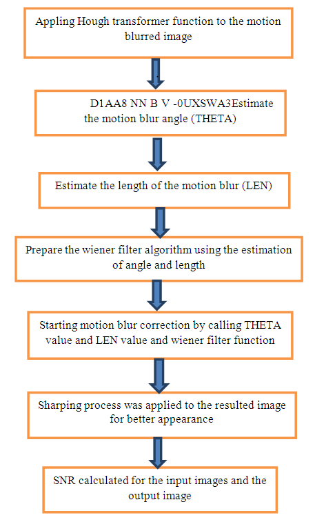Block Diagram 1. Illustrate the main methodology process

2.2. Motion Blur Angle Estimation Algorithm

a) Performing Median Filter before restoring the blurred image and Display the input image.

b) Converting image from spatial domain to frequency domain.

c) Compute the log spectrum of F (u, v).

d) Convert the image to Cestrum (spectrum (IFT)) domain Compute the inverse Fourier transform of log spectrum.

e) Finding the edge map of the image in cepstral domain of step d.

f) Let theta min and the theta max be the minimum and maximum values of the motion blur angle.

g) Calling Hough transform to initialized the accumulator array.

h) Finding first maximum in the accumulator.

i) Storing first maximum in the array.

j) Saving the original accumulator array.

k) Find the peak in Hough transform (the maximum value in accumulator array) which is perpendicular to the motion blur angle.

l) Iterating 10 times to find 10 highest angle values.

m) Calculate the possible values of THETA.

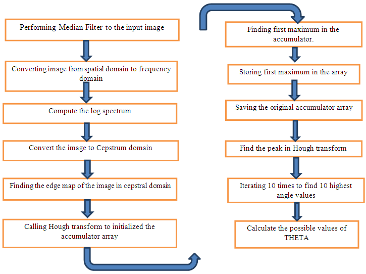Block Diagram 2. Illustrate motion Blur Angle Estimation Algorithm

2.3. Motion Blur Length Estimation Algorithm

a) Performing Median Filter before restoring the blurred image and Display the input image.

b) Converting image from spatial domain to frequency domain.

c) Compute the log spectrum of F (u, v).

d) Convert the image to Cepstrum (spectrum (IFT)) domain Compute the inverse Fourier transform of log spectrum.

e) Rotate the cepstral by the estimated angle in the inverse direction.

f) Convert the 2-D matrix of step e to 1-D by taking the averages of columns.

g) Find the distance of first negative peak from the origin which is corresponding to motion length.

h) If Zero Crossing found then return it as the blur length

i) If Zero Crossing not found then find the lowest peak Calculating the blur length using Lowest Peak

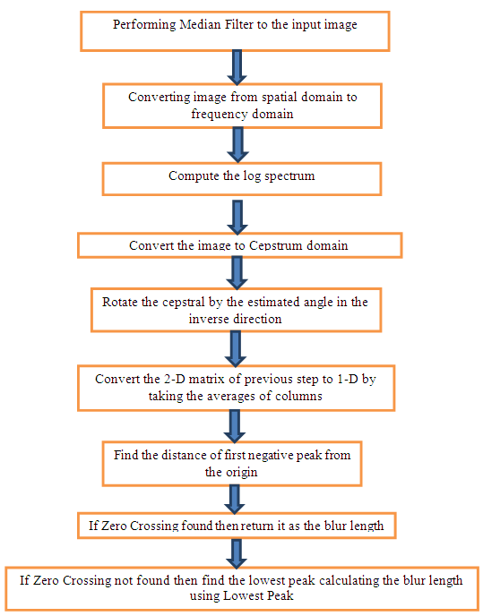Block Diagram 3. Illustrate motion Blur length Estimation Algorithm

3. Result

A new method for MRI motion blur correction on the personal computer (PC) side using MATLAB program had been developed, the resulted images and the measured values will be discus in this chapter.

To assess the overall impact of the using wiener filter in MRI image motion blur, the expected motion blur angle and motion blur length were estimated for more details Hough transform was used in line detection, ten different expected angles and length of motion blur were estimated.

According to the different measured angles and lengths motion correction was applied by wiener filter ten times, the resulted images were treated by sharpening filters and SNR were measured for all corrected image in order to compare which estimated angle and length were result a better a appearance.

For the ten different motion blur angles and lengths in coronal brain MRI image, the correction method results illustrated in the following figures, every one figure include the original image beside the corrected image in order to compare the different angles and length values restoration and their effect in the original corrupted image.

Then the same algorithm has been used for another sagittal and axial MRI motion blur image and the resulted corrected image has been illustrated following the coronal image figures, different angle and length for motion blur images has been estimated and accordingly different result was observed.

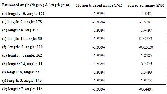
3.1. Coronal Sections

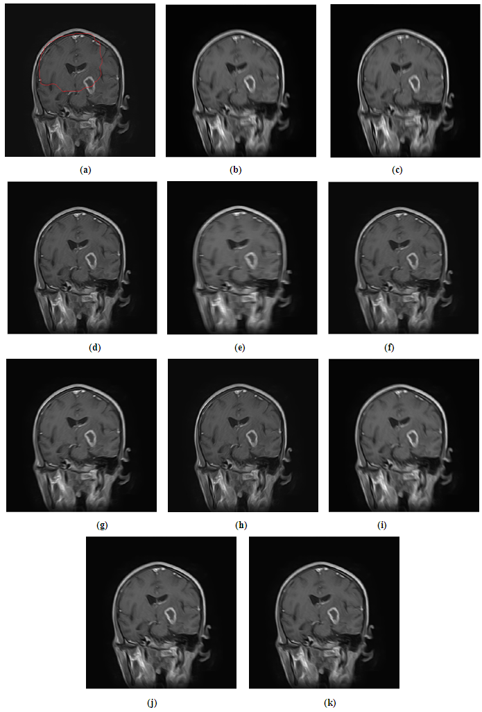Figure 1. (a) original image, (b,c,d,e,f,g,h,i,j,k) describe the motion blur correction images according to the following estimated angles and lengths as demonstrated in the table

The following table includes the estimated SNR for coronal corrected image in different angles and lengths comparing with the motion blurred image.

Table 1. Comparison between SNR of motion image and corrected image (coronal image)

Coronal sections discussion

By the visual inspection and consultation of radiologist and senior technologist comparing the original motion blurred image and motion corrected image. There is some anatomical structure were going to be diagnosable and clear more than before correction specially in angle 99 fig (5.2) and angle 112 fig (5.1) with the same length 11.

The table (1) above contains the ten corrected image with their angles, lengths and SNR. Angle 99 image (c) had the maximum SNR value in the table which determines that it has the better motion blur correction even by the visual inspection the correction was clear and given clear result in the coronal brain MRI image, image (d) with angle 173 and length 5 had the minimum SNR value hence lowest degree of motion blur correction. For the remaining corrected image they gave some degrees of correction but different values of motion distortion was remained in the image and that is why the correction algorithm take different value of expected angles and lengths. By the visual inspection comparing the original motion blurred image and motion corrected image. There is some anatomical structure was going to be diagnosable and clear more than before correction specially in angle 99 and angle 112 with the same length 11.

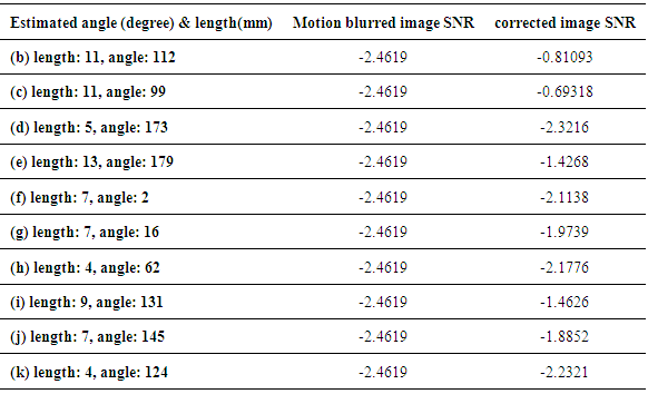
3.2. Sagittal Sections

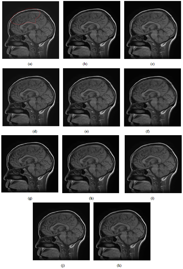Figure 2. (a) original image, (b,c,d,e,f,g,h,i,j,k) describe the motion blur correction images according to the following estimated angles and lengths as demonstrated in the table

The following table include the estimated SNR for sagittal corrected image in different angles and lengths comparing with the motion blurred image.

Table 2. Comparison between SNR of motion image and corrected image (sagittal image)

Sagittal sections discussion

Also in the sagittal image the visual inspection and consultation of radiologist and senior technologist comparing the original motion blurred image and motion corrected image. There is some anatomical structure were going to be diagnosable and clear more than before correction specially in image (c) angle 173, and image (e) with angle 2, image (f) with angle 21 and image (h) with angle 110. The table (2) above contain the ten corrected image with their angles, lengths and SNR. Angle 21 image (f) and angle 110 image (h) had the maximum SNR value in the table which determine that it has the better motion blur correction even by the visual inspection the correction was clear and given clear result in the sagittal brain MRI image. For the remaining corrected image they gave some degrees of correction but different values of motion distortion was remained in the image and that is why the correction algorithm take different value of expected angles and lengths.

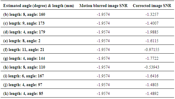
3.3. Axial Sections

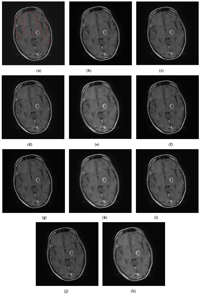Figure 3. (a) original image, (b,c,d,e,f,g,h,i,j,k) describe the motion blur correction images according to the following estimated angles and lengths as demonstrated in the table

The following table include the estimated SNR for sagittal corrected image in different angles and lengths comparing with the motion blurred image.

Table 3. Comparison between SNR of motion image and corrected image (axial image)

Axial sections discussion

Finally in the axial corrupted image also by visual inspection and consultation of radiologist and senior technologist comparing the original motion blurred image and motion corrected image. There is some anatomical structure were going to be diagnosable and clear more than before correction specially in image (b) angle 172, and image (c) with angle 178, fig (5.15). The table (3) above contain the ten corrected image with their angles, lengths and SNR. For the remaining corrected image they gave some degrees of correction but different values of motion distortion was remained in the image and that is why the correction algorithm take different value of expected angles and lengths.

4. Conclusions

In this study, a motion blur correction algorithm, used to assess coronal, sagittal and axial image for the MRI brain corrupted with rigid motion result to phase mismaping. Wiener filter was taken as the main algorithm in the correction procedure. According to ten different angles and lengths estimated before starting the correcting procedure. The correction algorithm achieved the best results which lead to clear appearance in anatomical brain feature and remove the motion blur which can obscure very important details. Although the corrected image by wiener filter gave a best result, it suffering some degree of unsharpeness, application of sharpening filter was needed and it gave better results. Motion blur in sagittal image result in highly degree of correction by the algorithm in the research. Since more than five images according to the different degree of angle and length estimation was totally corrected.