1. Introduction

Although physiological monitoring devices such as pulse oximeters and electrocardiogram (ECG) monitors have been in use to a large extent in the hospital environment, and to a much smaller degree in the private home or in assisted care facilities, such devices typically comprise sensors attached to the body, with the patient tethered by wires to the accompanying electronics, which in turn are mounted on a stand or placed on a table alongside the patient bedside. New devices that integrate on-body sensors and accompanying electronics into a small body-worn unit are currently in development, with first generation units now undergoing initial deployment. Combining the sensor functions and support electronics into a single unit removes the patient tether but still requires the device to be periodically returned to healthcare professionals for data offloading, or alternatively, requires patient interaction with the device for status checks and periodic data uploads.

Next generation on-body devices may include a wireless link to a nearby gateway, which in turn may be connected through various means back to a medical monitoring center. One such example that was based on the analysis presented herein can be found in [1]. In addition to removing the burden from the patient to interact manually with the device for data uploads, the presence of the wireless link enables additional functionality to be realized. With the benefit of continuous wireless connectivity, real-time alerts and data snapshots may be automatically transmitted to the medical team for immediate analysis. Such a system is depicted in Figure 1. Note in the figure inset the indoor “short-haul” communications link between the body-worn device and the notional gateway. This paper will describe the indoor short-haul link. A discussion of the “long-haul” link, from the house to the monitoring medical center, is presented in [2].

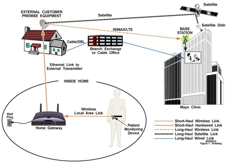Figure 1. Complete Radio Frequency Link from Patient at Home with Body Worn Health Monitoring Device to Monitoring Station Located in Medical Center with Three Long-Haul Link Options

Such a wireless communications link from an on-body biomedical device operating in an indoor environment requires consideration of several design elements. Technical requirements such as the optimum frequency at which to operate the link, the data rate needed to transmit physiological data within the required time frame, and maximum device run time between battery charging cycles, or battery replacements if primary (non-rechargeable) batteries are used, all need to be balanced against non-technical considerations. For example, regulatory requirements influence frequency and data rate options, whereas component availability and cost constraints often affect choices made that in turn directly constrain battery and run time options.

Two key elements that have a strong influence on the performance of the short-haul wireless link are the on-body device antenna performance, and operational boundary conditions generated by the indoor propagation environment. Several design considerations will be examined in the sections that follow, with special emphasis on these critical items.

1.1. Aims

Requirements for the addition of a wireless capability to an on-body medical device include minimizing the size increase over the basic (non-wireless) on-body device design, and maximizing the wireless coverage within the indoor environment. Additionally, the design needs to be conservatively planned to maximize the chances for a successful transmission by minimizing nulls in the on-body device’s antenna radiation pattern. Further, the design should support coverage within a typically sized private home and should be scalable to accommodate larger structures and multistory dwellings.

An additional requirement for the proposed system includes support for three transmission modes that include: 1) a ping mode for system status and periodic functional verification of the wireless link; 2) an alert triggered by a physiological event; and 3) a snapshot of measured physiological data immediately preceding the alert event. The data snapshot in particular affects the data rate requirements, which in turn impact antenna performance.

1.2. Structure of the Paper

In Section 2 we will first present the impact that the size of the on-body device has on the design of its antenna by exploring effects on antenna efficiency, quality factor, and usable bandwidth, followed by an analysis and simulation results of the human body’s interaction with the antenna. Section 3 will present the indoor propagation and coverage expectation for a private home environment that would typically be encountered by the wireless on-body biomedical monitoring device and gateway system. Finally, Section 4 will present a design example including test results of the on-body device and a corresponding gateway in a home environment.

2. On-Body Device Antenna

Antenna options for on-body medical devices are very limited due to the desire to minimize device size and the need for an omnidirectional radiation pattern. A wide range of frequencies are used for on-body (or in-body) medical devices, including: the Medical Device Radiocommunications Service (MedRadio) from 401 MHz to 457 MHz; the Wireless Medical Telemetry Service (WMTS) in the 608 MHz to 614 MHz, 1395 MHz to 1400 MHz, and 1427 MHz to 1432 MHz frequency bands; the new Medical Body Area Networks (MBAN) frequencies at 2360 MHz to 2400 MHz; and the ubiquitous 900 MHz and 2.4 GHz Industrial, Scientific, and Industrial (ISM) bands. Given these frequency options, the wireless link between the on-body device and the gateway will most likely need to operate between 400 MHz and 2.4 GHz. With an on-body device maximum dimension of 1.5”, the resulting antenna electrical size will be between 0.05 λ and 0.30 λ, where λ is the free space wavelength for a given frequency. At the lower frequency range an antenna of this dimension is well within the < 0.1 λ size that is typically defined as “electrically small”. Such antennas are generally difficult to impedance match for all but a very narrow band of frequencies, and suffer from poor radiation efficiency. Although the higher frequency range should be less sensitive to these performance issues, the impact of the body on the radiation pattern increases with frequency.

2.1. Antenna Efficiency, Q, and Bandwidth

We first examine the lower frequency range noted in the previous paragraph, which implies an electrically small antenna. One antenna performance parameter that is significantly affected by an electrically small antenna is the antenna efficiency . Antenna efficiency is defined as the ratio of the power radiated by the antenna to the total power input to the antenna, and can be expressed as the ratio of the antenna radiation resistance (R_r) to the total antenna resistance (R_a) where R_a includes the radiation resistance and ohmic (conductor) losses.

The radiation resistance for an electrically short dipole can be expressed as [3]:

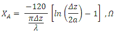
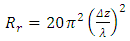, Ω; where Δz is the dipole length, and λ is the free space wavelength.

And the ohmic resistance R_Ohmic, for a circular cross section of wire with radius a and surface resistance R_S is found by [3]:

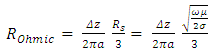, Ω; where R_S is the surface resistance, a is the radius, µ is the permeability, and σ is the conductivity of the wire, and ω is the radian frequency.

Combining these expressions gives the short dipole antenna efficiency as:

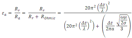Figure 2 illustrates the resulting efficiency for an antenna made from copper, whose conductivity is σ = 5.7 X 10⁷ (S/m), limited to a maximum length of 1.5”, and conductor radius of 0.007”. Clearly, the antenna efficiency at the lower end of the frequency range under consideration is quite poor, which in addition to constraining the communications range between the on-body device and the gateway, as well as degrading battery life, also results in a poor quality factor (Q) for the antenna. Note however that the lower Q may be advantageous since it may reduce the antennas sensitivity to impedance variations from interactions with the local environment (i.e. coupling to the body).

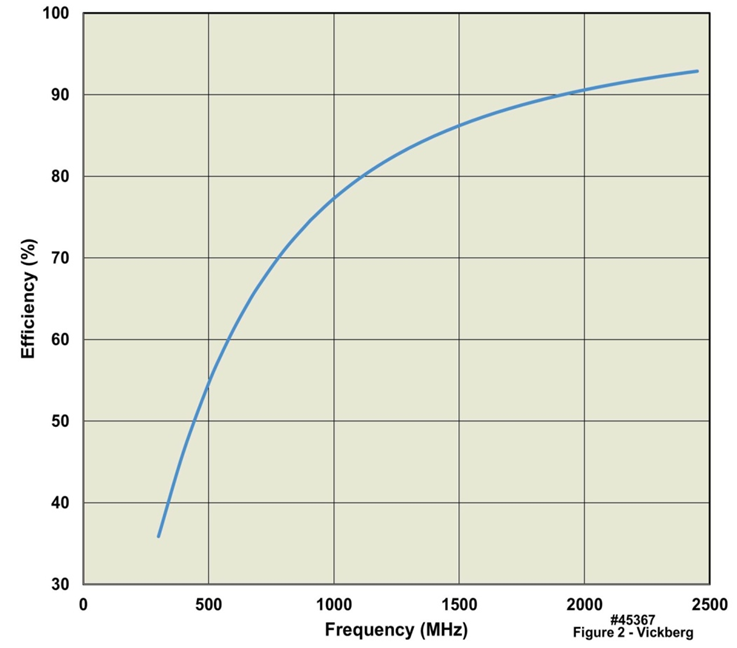Figure 2. Antenna Efficiency for Copper Wire Short Dipole 1.5" (38 mm) Long and with 0.007” (0.2 mm) Radius

The antenna Q relates to its usable bandwidth, and is defined as the total energy stored by the antenna divided by the power dissipated per cycle. The energy stored by the antenna is represented by the reactive component (X_A) of the antenna’s impedance, whereas the power dissipated is represented by the total antenna resistance R_a. For an electrically short dipole, X_A is found using the expression below [3], and R_A is found using the expression given above for efficiency.

The estimated Q and usable bandwidth (bandwidth here is estimated as 1/Q) for an electrically small dipole operating in free space, using the dimensions from the efficiency example given above, is shown in Figure 3.

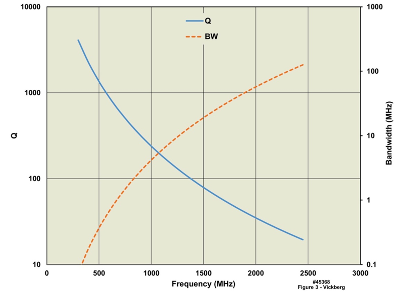Figure 3. Short Dipole Antenna Q and Bandwidth for Copper Wire Antenna 1.5” (38 mm) Long and 0.007” radius

To place the bandwidth results into perspective, if the wireless link between the on-body device and the gateway were to be operated at low power under FCC Part 15 rules, using for example one of the ISM band frequencies, the bandwidth requirement would be determined by the amount of data that needed to be transmitted and the duration during which the data transmission needed to occur. By FCC rules, this low power transmission scenario is limited to approximately 1 mW. Such power levels may be sufficient for situations in which the on-body device and gateway are located in close proximity, e.g., within the same room. When longer transmission distances are needed, or when there may be more signal loss due to building construction, obstructions, or nulls in the antenna radiation pattern, higher transmission power may be required. FCC Part 15 rules also allow for higher power operation but place additional requirements on the modulation type and spectral components of the transmitted signal. One such requirement for the higher power operation is that the signal occupies a minimum 500 kHz 6 dB bandwidth. From Figure 3, this bandwidth requirement establishes a lower limit to the carrier frequency to be between 500 MHz and 600 MHz.

2.2. Human Body Impact on Antenna Radiation Pattern

Ideally, the antenna radiation pattern for the on-body device would radiate in an omnidirectional pattern so that the orientation of the wearer would not affect the ability to close the communications link between the on-body device and the gateway. For an antenna operating in free space, a vertically polarized dipole presents such a radiation field pattern. However, when such an antenna is placed in close proximity to the body, several interactions between the body and the antenna may occur, depending on the separation distance between the body and antenna, as well as on the operating frequency. Radiation fields from the antenna may pass through the body, reflect and diffract from the body, or travel along the body surface.

To quantify the electromagnetic energy that may pass through the body, we first consider the attenuation that the body presents at a given frequency. For a general dielectric material, the propagation constant (γ) of a plane wave is given as:

where the real part of γ, α, is the attenuation constant and β is the phase constant. The attenuation constant represents the losses and is given by [4]:

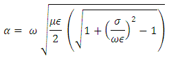Where (μ) is the magnetic permeability, (ε) is the electric permittivity, and (σ) is the conductivity of the dielectric material.

The magnitude of the electromagnetic wave that passes through the body may be determined from the number of skin depths that the body represents for a given frequency, where:

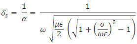Note that by definition, is the depth at which the magnitude of the electric field is diminished by a factor of 1/e, resulting in a reduction of the original signal strength to approximately 37% of its original value. A plot of over the frequency range of interest is shown in Figure 4, in which the average dielectric constant of the body is taken as that of water, which is approximately equal to 80, and an averaged conductivity of approximately 1 S/m, are assumed.

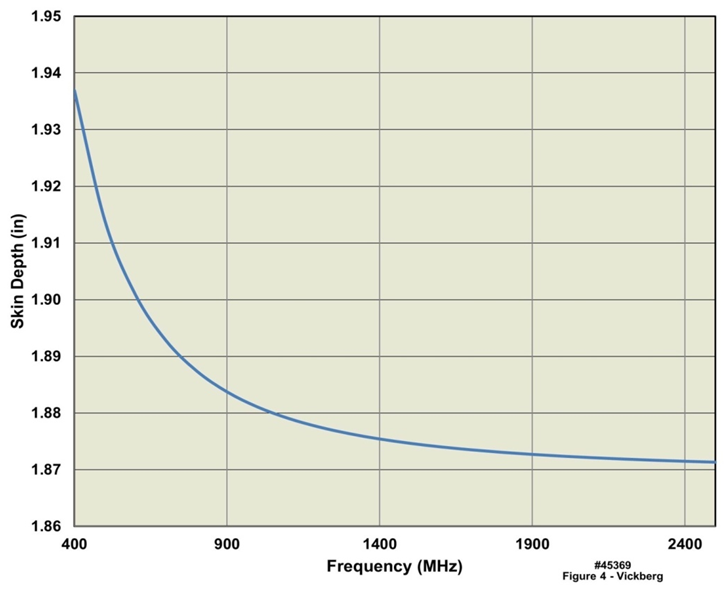Figure 4. Skin Depth for a Dielectric Material Approximating a Torso with a Relative Dielectric Constant of 80 and a Conductivity of σ = 1

From Figure 4, the skin depth over the frequency range of interest is nearly constant at approximately 2 inches, giving 4.75 skin depths for an average torso dimension of 9.5 inches from front to back, which is equivalent to 41 dB of loss. Given the estimated loss through the body over the frequency range it is very unlikely that the primary communications path will be through the body.

To evaluate the non-transmission effects of the body on the antenna radiation pattern we first adopt an analytical approach in which the torso is represented by a perfectly conducting cylinder. As shown in Figure 5, the model includes a vertically polarized dipole aligned to the cylinder axis and placed in close proximity to the cylinder.

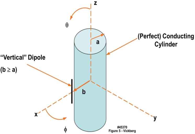Figure 5. Vertical Dipole near a Perfectly Conducting Cylinder

To approximate the radiation pattern produced by this configuration, Jordan and Balmain [5] provided a closed-form solution to this problem, as given below.

where 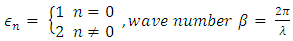, Jn is the Bessel function of the first kind, and Hn is the Hankel function of the second kind.

Using this expression, we calculated the radiation patterns over a frequency range from 300 MHz to 2.4 GHz, with a = 0.25 m (9.8”), and b = 0.2525 m (10”), where b is measured from the central axis of the cylinder, which places the antenna approximately 0.2” (5 mm) from the cylinder surface. The resulting radiation patterns are plotted in Figure 6. From the figure, the phi = 0 degree point represents radiation from the front of the body (assuming that the on-body device is located on the front of the torso) and the ± 180 ° values represent the radiation from the back. Note the pattern falloff to the sides and around the back, which increases as a function of frequency. Over the frequency range modeled, at 90 degrees from boresight, the pattern level falloff increases by 5.8 dB from the lowest to the highest frequency and at 180 degrees the falloff increases by 30 dB over the frequency range. Based on this analysis, the lowest possible frequency would be the best option if no other considerations are taken into account. Although not shown, a similar analysis of a horizontally oriented antenna yields a similar result.

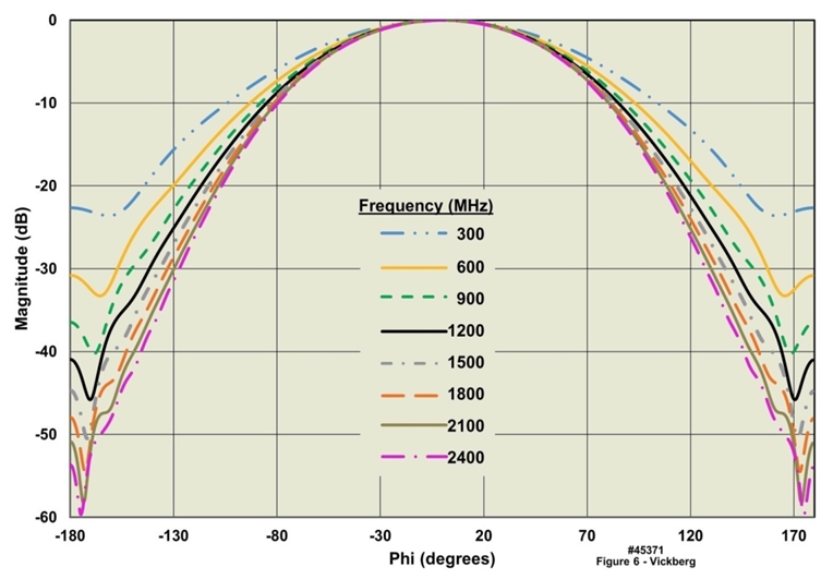Figure 6. Radiation Pattern versus Frequency from a Vertical Dipole near a Perfectly Conducting Cylinder; (a = 0.25m, b = 0.2525m, θ = 90º)

2.3. Simulations

The analysis described in the previous section was based on a simplified model of the human torso, which was represented as a perfectly conducting cylinder with dimensions approximating those of a typical adult. A full analytical analysis based on a more realistic model is not practical using a similar approach; however, current 3D electromagnetic simulation tools, in particular CST Microwave Studio, includes a numerical model of a complete human which includes electrical properties of the various tissue types for a variety of frequencies. Figure 7 shows the antenna location, “Hugo” body model, coordinate system, and far field antenna radiation pattern for the simulations that follow. Note from the figure, the “front” facing direction for Hugo is aligned along the y axis and is located at 270 degrees for the 2D plots.

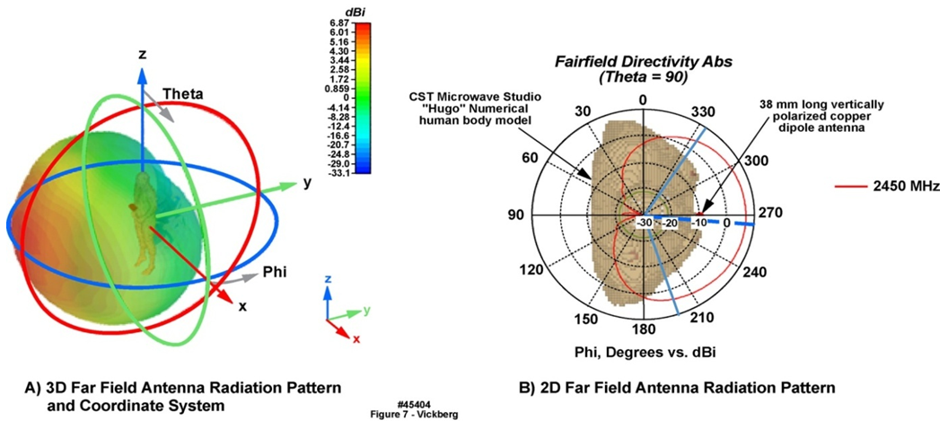Figure 7. CST Simulation of a Vertically Polarized Dipole Antenna Placed Directly in Front of the CST Hugo Human Body Model. A) 3D Far Field Antenna Radiation Pattern and Coordinate System, B) 2D Far Field Antenna Radiation Pattern

Using the Hugo model with the antenna orientation given above, and a 1.5” (38 mm) copper wire dipole antenna representing the maximum-case dimension for the body worn unit, several simulations were completed in which the antenna-to-body distance was varied for three frequencies. From these simulations, the effects on the radiation pattern and antenna impedance were evaluated. Figure 8 shows the radiation pattern for four distances, 2.5 mm, 20 mm, 40 mm, and 50 mm. For each of these positions the radiation patterns at 450 MHz, 900 MHz, and 2450 MHz were simulated, where the frequencies selected were based on the frequencies available from the Hugo body model. Note from the figure that all radiation patterns are shown in comparison to the same dipole antenna radiating in free space. The Hugo model was removed from the simulation for the free space dipole reference. All radiation patterns are plotted in terms of directivity, which is defined as the ratio of the radiation intensity in a given direction from the antenna to the radiation intensity averaged over all directions [6], for the given antenna, frequency, and location. Realized gain, through impedance matching, is more appropriate for system analysis and will be considered in the impedance results section that follows. Note that for panel ‘A’ the 450 MHz and 900 MHz patterns are very similar, with 10 to 18 dB less falloff in directivity, as compared to the 2450 MHz case, at the 90 degree back side of Hugo (recall that 270 degrees faces forward). At the other end of the separation range examined, i.e., 50 mm, panel ‘D’ shows the 900 MHz and 2450 MHz cases with very similar performance, whereas the 450 MHz case still shows 5 dB less falloff than the 2450 MHz case. In the middle range, 20 mm, panel ‘B’ shows that the 900 MHz case falls between the 450 MHz and 2450 MHz examples. Overall the trend observed from the analytical analysis from the previous section holds; that is, as the frequency is reduced, the impact on the antenna radiation pattern, as it pertains to omnidirectionality, by the body is also reduced.

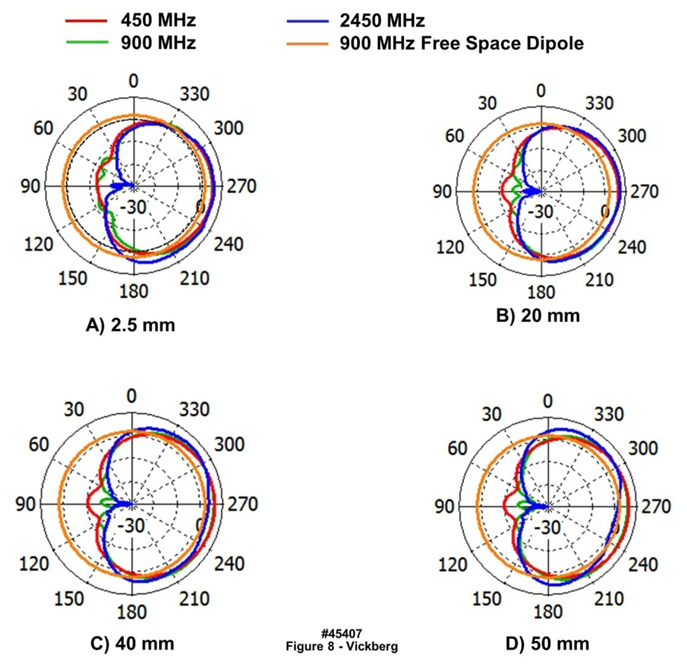Figure 8. Simulated Directivity for 38 mm Diameter Vertically Polarized, Copper Dipole Antenna Placed at Various Distances from the Human Body

In addition to the variation in the falloff in the directivity towards the back of the radiation patterns with increasing frequency, the forward directivity also varies across the range of frequencies and distances studied. One figure of merit that may be used that includes both of these radiation pattern “features” is the front to back ratio. To simplify the comparison, the directivities at 270 degrees and 90 degrees were recorded, with the difference plotted below in Figure 9. Note once again that the frequency dependent effects on the radiation pattern (for the given fixed length antenna) are well illustrated; i.e., as the operating frequency is increased, the potential to have dropouts in coverage when the transmission path is behind the body is greatly increased due to the effect on the antenna radiation pattern. Note from the figure, at 30 mm separation distance between the “on-body” device and the body there is over 25 dB of difference in directed power from the lowest frequency studied (450 MHz) to the highest frequency (2450 MHz). Recall that front to back ratio is used here only to illustrate the differences in the radiation patterns. If the edge of coverage is determined by the radiation pattern peak, then directions in which the pattern is reduced (pattern nulls), which are not necessarily limited to the back of the pattern, that were used to calculate the front to back ratio, would fail to close the link. Good engineering practice would normally account for this reduction by adding design margin. However, in general, as the variations between the pattern peaks and minimums increases, i.e. increased front to back ratio, additional margin is needed to compensate for the difference and the total effective coverage area for a given frequency is reduced.

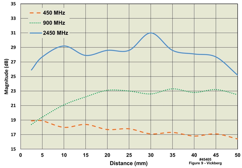Figure 9. Comparison of Simulated Front to Back Ratio for Vertically Polarized 1.5” (38 mm) Copper Dipole Antenna Placed at Various Distances in Front of the Human Body

In addition to the radiation patterns presented above, the antenna impedance was also simulated for all of the cases presented; Figure 10 shows the simulation results. As depicted in panel ‘A’ of the figure, the real part of the impedance appears to be well behaved over the frequency range and the antenna to body separation distances simulated. At 1.5” (38 mm) antenna length, the 2450 MHz case represents a wavelength of 31% λ and the simulated impedance is close to the expected value for a dipole antenna approximately one quarter wavelength long. Similarly, the 900 MHz and 2450 MHz cases are electrically short and as expected have a real part of the impedance value that is relatively low. This low impedance, along with the increasing imaginary part shown in panel ‘B’, sets a lower bound on the usable bandwidth of the short dipole due to impedance matching limitations. Note that the antenna patterns shown above can be interpreted as gain plots only if impedance matching is applied. Impedance matching is also necessary to limit loss of signal between transmitter/receiver circuits and the antenna. Without such matching, transmit power would be reduced. Compensating for such loss by increasing transmit power will consume more battery power, and receive sensitivity will be reduced.

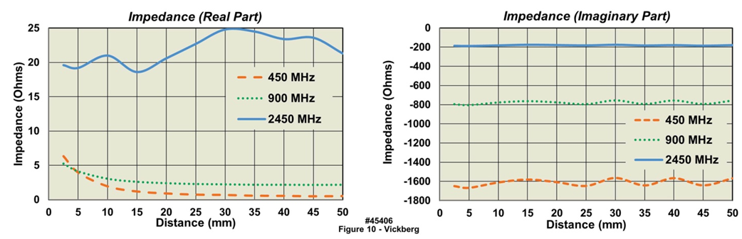Figure 10. Comparison of Simulated Impedance Values for Vertically Polarized 1.5” (38 mm) Copper Dipole Antenna Placed at Various Distances in Front of the Human Body

3. Considerations for Indoor Propagation

In addition to the impact that the body has on the short-haul link performance, the indoor environment that the link is operated within also plays a significant role in the performance and coverage of a given on-body device and gateway design. For brevity, we focus on the far field propagation for the indoor wireless link analysis. Any interactions between the antenna and nearby structures, such as furniture, walls, the floor, etc., that the on-body device may be in close proximity to, are not considered in this analysis.

As an electromagnetic wave moves through space it interacts with objects in the environment by reflecting, scattering, or passing through (transmission) the materials encountered. Analysis of the complex interference environment that results from these interactions is nontrivial for all but the simplest cases and is variable as persons and objects are moved within the volume analyzed. To model such an environment the path loss exponent from Friis formula, given below [7], for free space propagation is modified to account for the increased losses found in the typical indoor propagation environment:

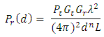where is the power received, is the power transmitted, is the transmit antenna gain, is the receive antenna gain, and λ is the free space wavelength. The variable dⁿ represents the separation d between transmit and receive antennas, with the path loss exponent n [8] set equal to 2 for free space. Note that n for indoor propagation has been found to cover a range of values of approximately 1.8 to 4.8 [8], [10], [11] for various building types and constructions. Finally, L is the sum of the losses due to a variety of sources such as multipath and attenuation, as well as non-propagation dependent system losses. Note from the above that gain is more appropriate for system analysis than directivity, and is defined as the ratio of the radiation intensity to the power accepted by the antenna, and can be expressed as the antenna radiation efficiency times the directivity [9].

Setting the antenna gain to 1, which is a reasonable approximation given that an omnidirectional radiation pattern is desired, causes the antenna gain terms to drop out of the received power calculation. Rearranging the remaining terms, limiting loss components to only spreading of the electromagnetic wave and interactions in the propagating environment, the path loss (PL) can be expressed as:

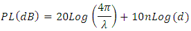Taking an average value of 3.3 for n, the path loss expected for three frequencies over distances of a typical residential house are plotted in Figure 11. Note that between the frequency extremes evaluated (300 MHz to 2450 MHz) there is a nearly constant 18 dB difference in path loss for the separation distances between the on-body device and gateway, as shown in the figure. In this case the lower frequency bound of 300 MHz was chosen simply to illustrate the trend as the frequency is lowered. Further, between the two common ISM bands, 915 MHz and 2450 MHz, there is also a very significant difference of approximately 10 dB in path loss.

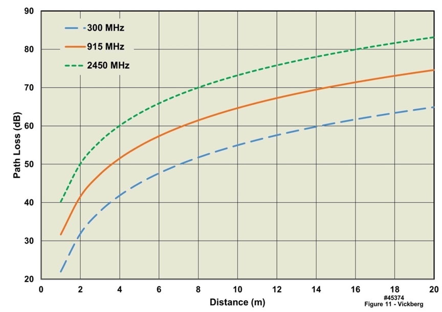Figure 11. Indoor Path Loss (propagation loss exponent = 3.3)

3.1. Indoor Coverage Estimates

The maximum distance for a successful wireless link between a given gateway and the on-body device is designated as the gateway’s coverage area and is based on numerous transmitter, receiver, and propagation environment parameters. Some parameters, such as allowable transmit power and antenna gains, are limited by FCC rules, whereas the propagation environment is largely affected by building construction materials, objects in rooms, humans, etc., which in turn impact attenuation, reflections, scattering, etc. and the resulting multipath environment. On the receiver side, the minimum signal to noise ratio sets the limit for the receive power required to recover the transmitted message successfully.

For digital modulation, which would be the likely choice due to the data transmission needs of body-worn physiological monitoring devices, and to leverage existing wireless protocols and component availability, the acceptable bit error rate (BER) is used to set the limit for a successful transmission. Although consumer electronics applications accept BER as “low” as 10^-3 (1 error for every 1000 bits transmitted) for Bluetooth, or 10^-5 for WiFi, we chose a more conservative BER of 10^-6 to increase system robustness for medical alerts.

Translation from BER to equivalent SNR is dependent on the modulation technique and is related to the ratio of the amount of energy-per-bit (E_b) to the noise (N₀), normalized to a one Hertz bandwidth, and the ratio of the bit rate (R) and bandwidth (B) of the transmitted signal.

For a BER of 10^-6, SNR_min falls in the range of 10.5 dB to 15 dB for the simple digital modulation techniques, such as frequency shift keying, that would likely be used for biomedical applications [1].

3.2. Path Loss

In addition to the frequency dependent indoor path loss considered above, maximum allowable path loss (MAPL) estimates the total loss that can be accepted while still maintaining SNR_min. Substituting the receive power requirements as determined by SNR_min, and the receiver noise performance into Frii’s formula, and solving for the loss term, yields the expression for maximum loss given below:

where B is the receiver bandwidth in Hz, which is related to the data rate requirements; F is the receiver noise factor, defined as the receiver input signal to noise ratio divided by the receiver output signal to noise ratio; k is Boltzmann’s constant; T is the system temperature in degrees Kelvin; and L_max is the MAPL.

Based on published specifications for commercial radio frequency integrated circuits (RFIC) considered for this analysis, and accounting for components and printed circuit board traces between the antenna connection and the input to the RFIC, we estimated the total receiver noise to be 15 dB, which is equal to a noise factor F of 31.6. Assuming omnidirectional coverage, values G_t and G_r are set to 1 for unity gain. To maximize battery time, P_t is set to the low power mode “maximum”, which is limited to -1.25 dBm based on FCC Part 15 rules. The bandwidth is set to 20 kHz based on several factors: 1) three axes of acceleration data, combined with; 2) non-diagnostic ECG; 3) an overhead component for data packetization; and 4) a compensation term for receiver pass band edge roll off [1]. Using these values, the maximum path loss is found to be .

From Saunders and Aragón-Zavala [12], the COST 231 propagation model is modified to include the effects of attenuation through walls, floors, and shadowing:

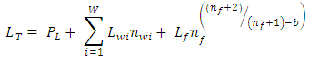where L_T is the total loss, represents the path loss determined above, is the loss for wall type i, is the number of walls of type i, is the loss per floor, n_f is the number of floors in the path, and b is an empirically derived factor which accounts for the observed nonlinear function of the number of floors [13].

Simplifying the previous equation for a single level house (including a basement) and combining with the indoor path loss model gives:

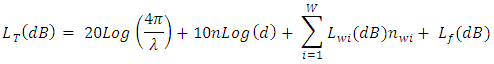Using wall loss and floor attenuation values from Saunders and Aragón-Zavala [12] and Dobkin [14], the total path loss for the two ISM band cases for which attenuation values were available, were calculated and are presented in Figure 12. From the figure, the total path loss for the single-floor three-wall 915 MHz case is within 2 dB of the no-wall and no-floor case at 2450 MHz.

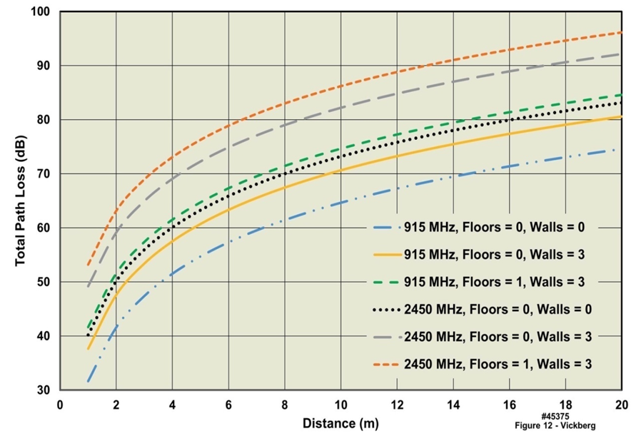Figure 12. Total Path Loss Including Wall and Floor Attenuation Examples

3.3. Coverage Estimate

Since most rooms include static objects such as furniture and other household items, as well as dynamic objects, such as the movement of people and pets, the real world presents a very complex and variable multipath environment. Such environments are subject to shadowing, which is the fading caused by changes in the scatterers for the different paths, depending upon the relative locations of the on-body unit and the base station. The previously defined (simplified) path loss model gives the median path loss, whereas the actual path loss includes a random component which accounts for the changing scatter environment observed from path to path. Since the random component of path loss can often be assumed to be a zero-mean Gaussian random variable, statistical methods are often used to characterize these types of environments.

The probability that the signal will exceed some threshold value L_T for a given distance d can be found using the complementary cumulative normal distribution function Q(t) [15].

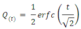Expressing Q(t) as a probability of coverage is given as:

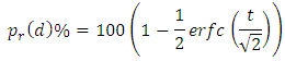where 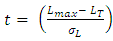, assuming L_T < L_max, σ_L is the standard deviation of the random part of the path loss, L_max - L_T is the fade margin for the system, and all values on the right hand side of this expression are expressed in dB.

Taking the location variable σ_L as 8 dB, based on estimates by Saunders and Zavala [12], and using the L_T value calculated above for the worst case scenario, which included three walls and one floor, the final coverage probability is shown below in Figure 13. Note from the figure that distances plotted represent those that might be encountered in a house of typical size, and for these distances there is a significant difference in expected coverage for the two ISM band frequencies evaluated.

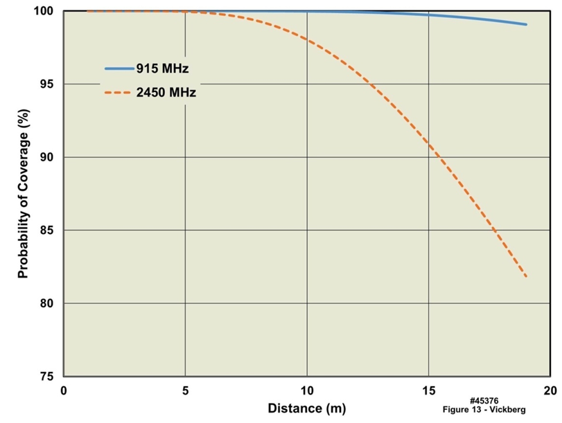Figure 13. Probability of Coverage for Low Power Short-Haul Wireless Link Operating Mode in an Indoor Environment Including Losses from 3 Walls and 1 Floor

4. Design Example

Based in part on the results described above, an on-body wireless physiological monitoring device and corresponding gateway were designed and are presented below. Key design requirements included minimizing the on-body device size and maximizing the indoor coverage area within the home environment.

The design process for the on-body device comprised three incremental steps which included: 1) a breadboard design, focused on the initial development of the radio frequency circuitry; 2) a reduced-size daughter board design, incorporating lessons learned from the breadboard design and allowing direct attachment to previously designed platform electronics hardware; and 3), a final prototype design combining these circuit functions into a single design. A custom antenna was also designed and fabricated, which ultimately had to fit inside of and work within the prototype package. Finally a gateway, which was used to receive the on-body device transmissions and forward the pings, alerts, and data over another communications path to a monitoring station, was also developed.

Selection of a frequency at which to operate the wireless link was based on several factors including 1) the desire to operate at the lower end of the frequency range analyzed and described above, to minimize the effect from the body on the antenna radiation pattern; 2) the availability of COTS components; and 3) limitations imposed by FCC regulations. Further, 1) due to the reduced antenna performance at the lower frequencies, i.e., a higher Q factor, decreased usable bandwidth and higher expected tuning sensitivity; and 2) while at the higher frequencies, e.g., 2.45 GHz, antennas exhibit higher front-to-back ratios (less omnidirectionality and lower probability of coverage at longer distances; 3) the 915 MHz ISM band was selected.

4.1. On-Body Device Antenna Design

Given the size constraint of the on-body device, any antenna structure selected for the 915 MHz frequency would be considered electrically small, or nearly so. Although the reactive part of the electrically small antenna impedance is typically high, some control may be realized with a bent monopole design, in which the monopole is bent so that it becomes parallel to its ground plane. Meandering introduces additional inductance which offsets the inherent capacitive reactance of a small monopole. The meandered monopole design implemented on a PCB offers several tuning mechanisms, including 1) the number of meanders; 2) the spacing between the meanders; 3) conductor width; and 4) for the case in which the antenna is a separate structure over another PCB, antenna substrate thickness and standoff distance between the antenna and the supporting PCB are also adjustable parameters.

The initial meandered monopole design was completed using a numerical electromagnetics code (NEC2) simulation tool, in which the antenna was subdivided into short wire segments. The Method of Moments was used to solve for the field components. The simulation tool determined both the far field radiation pattern and the impedance properties of the simulated structure. Once the initial design was completed, a full 3D analysis was conducted using CST Microwave Studio, which allowed planer structures such as printed wires to be quickly simulated over a wide range of variables. Figure 14 depicts a set of meandered monopole antennas fabricated on printed circuit board material. The parameters varied in this design included the number of meanders, line widths, and numerous locations for a shorting pin that could be used to remove meanders when tuning the antenna impedance.

Figure 14. Meander Line Antennas Printed on 6 mil Thick Printed Circuit Board Dielectric Material with 5, 10, 15, and 20 mil Wide Meander Traces and 11 to 33 Meanders

4.1.1. Meandered Monopole Antenna Test Results

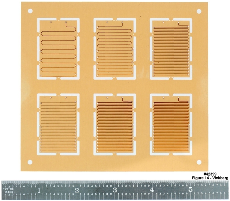
Using a mockup of the on-body electronics PCB, assembled on a blank PCB panel, as the supporting structure for the meandered monopole antenna substrate, the return loss of the meandered monopole antenna was measured in a free space environment. Several measurements were made using the various combinations of line widths, number of meanders, with and without the shorting pin at the end of the antenna, and after removing several meander lines. Figure 15 illustrates one such antenna optimized for free space operation. For this example, a standoff distance of 2.5 mm was established between the antenna substrate and PCB, and the antenna was not encased in a plastic housing. This specific example also employed a line width of 0.005”, a line spacing of 0.020”, and 13.5 meanders remaining after removing two meander lines. This version was self-impedance matched in that no additional matching components were used, which resulted in a 15 MHz 10 dB return loss centered at 915 MHz.

Figure 15. Measured Meandered Monopole Antenna Return Loss

The next step in the antenna characterization involved moving the assembly into an RF anechoic chamber where potential reflections from metallic benches and other objects in the test lab were not present. Two test configurations were conducted in this environment. The first study was the antenna under test by itself, mounted on a non-reflective mast. The antenna was positioned with its longer dimension in a vertical orientation, since this configuration was the expected orientation to be used in the final design. The antenna was then rotated through 360º as the radiation pattern was recorded.

To simulate the influence of the antenna next to a body, a second test was conducted with the antenna attached to a five gallon plastic pail containing a human tissue phantom material, which mimicked the electrical properties of the human body at the test frequency. The recipe used for the phantom material was from the FCC document “Evaluating Compliance with FCC Guidelines for Human Exposure to Radio Frequency Electromagnetic Fields, Supplement C to OET Bulletin 65.” The dielectric properties for this test were ε_r = 57_, and σ = 1.07 S/m. The recipe contained a mixture of 65% H₂O, 41.76% sugar, 1.21% hydroxyethyl cellulose, and 0.76% NaCl by weight. Figure 16 presents the test setup in the anechoic chamber, with the plastic pail positioned on the turntable using wooden stools at the same height as the receive antenna (not pictured) at the other end of the chamber.

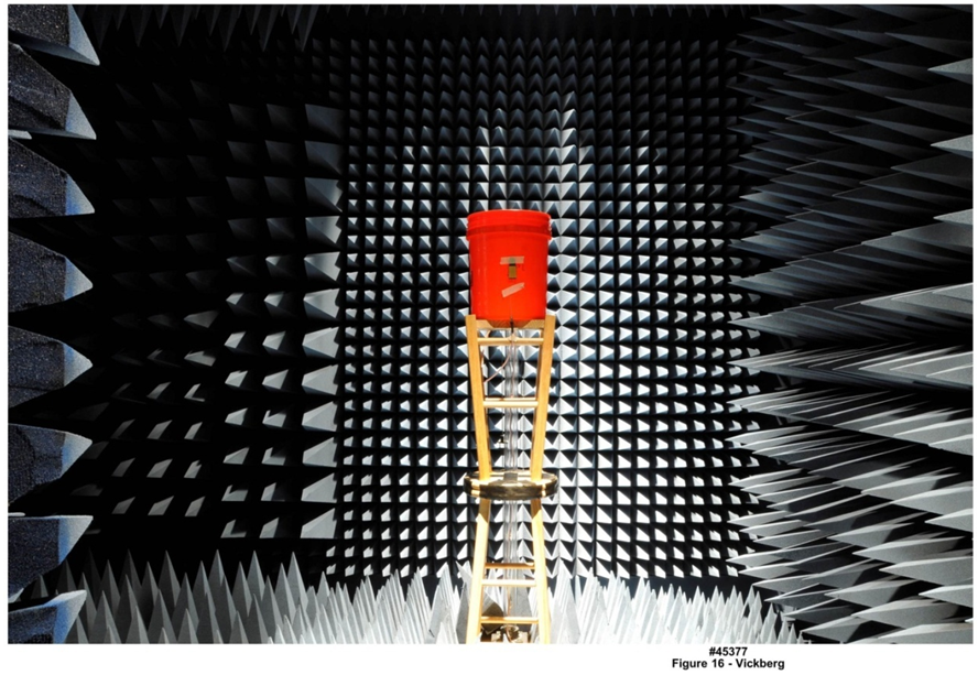Figure 16. Meandered Monopole Antenna Test in Anechoic Chamber with Plastic Pail Containing Phantom Material

Figure 17 presents the measurement results for the antenna under test in free space and against the plastic pail containing the phantom material. Note that, as expected from previous simulations, the antenna exhibits a nearly omnidirectional radiation pattern for the free space configuration but there are deviations caused, in part, by the small (in terms of wavelength) size of the ground plane. There is significant current flowing on the underside of the ground plane, which produces much of the radiation seen for angles between 90^o and 270^o. In addition there could be some radiation from currents flowing on the outside of the feed cable. However, the result against the pail containing the phantom material does not match the dipole in front of a conducting cylinder as calculated earlier in this manuscript; this result is not unexpected, as the monopole has a ground plane between it and the cylinder. Although the measured radiation pattern is not ideal, one “feature” of this pattern is that more energy is radiated towards the back than toward the front, which may help mitigate the situation when the wearer has fallen and is blocking the communications path with his body. Further investigation of these results is needed.

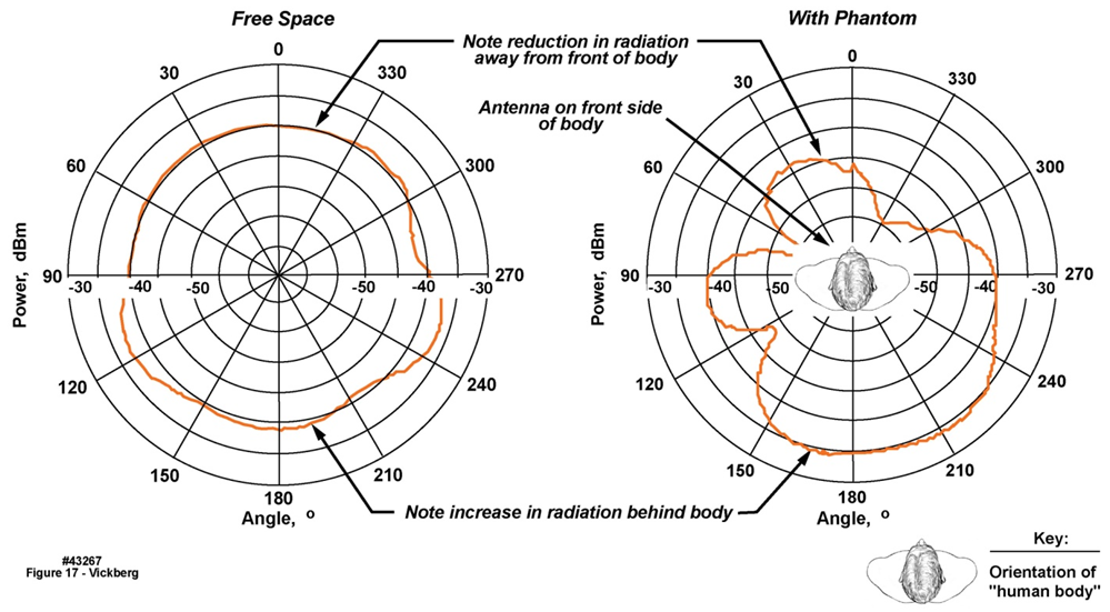Figure 17. Comparison of Radiated Signals versus Angle for Meandered Monopole Antenna in Free Space and Against Plastic Pail Containing Phantom Material

4.2. Prototype On-Body Device Design

Figure 18 shows a completed prototype design of the on-body physiological monitoring device housed in a clear polycarbonate case. The design pictured includes a second generation of the meandered monopole antenna that has been optimized (tuned) for operation within the case. Also pictured is a lithium polymer prismatic battery that was chosen to provide the current surges necessary for times in which the short-haul link transceiver is active. This design includes two three-axis accelerometers, a 1 GB data memory for logging all physiological data recorded during use, and an external port used to connect to additional circuitry and sensors for additional sensing functions such as ECG, pulse oximetry, or respiration, other as-yet undetermined add-on features, and/or test circuits.

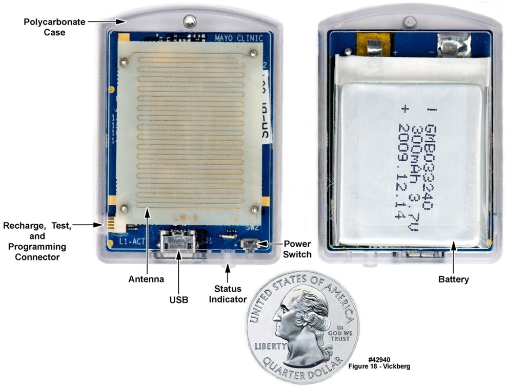Figure 18. Front and Rear Views of Final Form Factor Combined Short-Haul and Platform Electronics

4.3. Test Results

In addition to basic functionality tests, other critical tests for the on-body device and gateway included verification that transmit parameters met FCC Part 15 requirements, verification of run time tests using the selected battery, and coverage tests of the on-body device and gateway system in a residential setting.

4.3.1. RF Transmission Tests

Verification of transmission parameters was accomplished by direct connection of a power meter and spectrum analyzer to the output of the transceiver at a test point located on the output side of the matching network. Transmitter performance measurements were made at the band edges and band center frequency for four power level settings using an HP E4419B power meter, HP 8485A power sensor, 1 ft. long Sucoflex 104 cable with 3.5 mm connectors, and a coaxial DC block. Losses through the test cable and DC block were measured using an HP 8722ES network analyzer. Since the final meander antenna design was self-matching at 50 Ohms, results obtained from these measurements were easily translated to the final device results by including the antenna performance parameters, which were measured separately. After factoring in the meander line antenna performance, the final transmit power level fell below the maximum allowed by FCC regulations, as desired.

4.3.2. Battery Runtime Test

Beginning with a fully charged battery, the combined short-haul and platform electronics assembly was configured to run test pings only. For this test the short-haul circuit was configured to operate at maximum power setting. After four hours of continuous operation in this mode, the total energy required to recharge the battery was recorded and found to be 12 mAh. The ping transmissions were sent every six seconds during the test period. Based on this test, the estimated run time for the short-haul portion of the combined circuit was determined to be 2.5 days using the 180 mAh battery.

For a normal operating mode in which verification of “system ready” status is conducted every minute using an automated ping transmission, the total run time in this mode extends to 25 days. From this result and the known current requirements for the platform electronics, an estimated operating duration can be calculated for various operating configurations. Similarly, operating duration estimates for transmission of alerts and data snapshots can also be scaled based on these results, since they use the same transmission mode but for longer transmission times.

4.3.3. Coverage Test

A coverage test was conducted in a private residence using the combined short-haul and platform electronics circuit, along with the home gateway. For this test the transmitter was set to -1 dBm, 915 MHz, 36 kbaud, and frequency shift keying (FSK) modulation.

The test included four configurations, as indicated in Figure 19. Each test consisted of a verification that the home gateway successfully received a ping transmission from the short-haul circuit, by illuminating a “transmission received” acknowledgement indicator on the home gateway. Solid green dots in the figure above indicate the successful reception of the test transmission. This test confirmed that for this case, with the gateway located approximately in the center of the house, complete coverage was realized for the house size and floor plan indicated in the figure. Other home construction types and greater square footage may still result in gaps in coverage; for these instances multiple gateways will likely be needed.

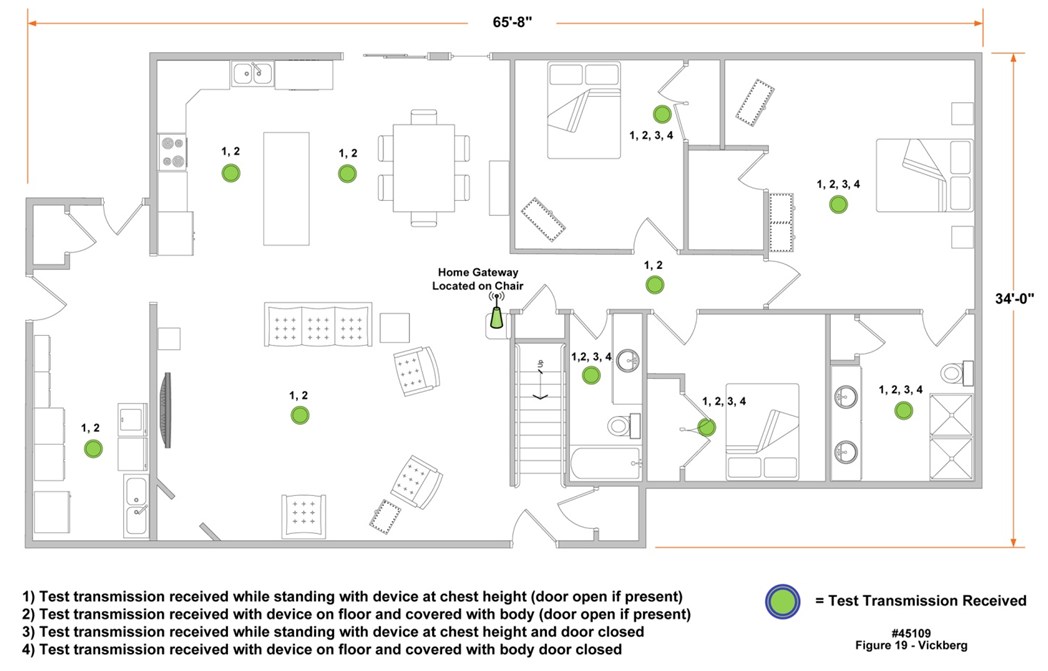Figure 19. Coverage Test Results using Short-Haul Circuit and Home Gateway

5. Discussion

As discussed and described above, from the numerous engineering parameters that must be considered when designing a wirelessly linked on-body biomedical monitoring device for use in a home environment, the frequency with which to operate the link has significant implications on antenna performance and indoor wireless link performance. Given the frequency dependent properties of the human body [16], it is not surprising that there is a frequency dependent effect on the radiation pattern of an on-body antenna as compared to its free space radiation pattern.

Of the two methods presented above that were used for analyzing these frequency dependent tradeoffs, the first method, a “clean slate” approach, demonstrated that the conducting cylinder, representing an “averaged” torso, had a very significant impact on a canonical dipole placed in close proximity to the cylinder surface. By approaching the antenna performance analysis without bias towards a specific frequency band, i.e. not limited to ISM band options, our analysis considered a wide range of frequencies. Comparable examples of work covering a similar frequency range were not identified in the literature. However, one example, based on the 2.45 GHz ISM band, did present a similar result. Sani et al. [17] showed the impact of the body on antenna radiation pattern at 2.4 GHz for two antenna types, a patch antenna and an inverted L. The inverted L produces a radiation pattern similar to the dipole studied above and serves as a comparable example.

Sani compared the free-space radiation pattern to the pattern obtained by holding their antenna in close proximity to the body, illustrating that the measured inverted L response, with the antenna located next to the body, yielded a 20 to 40 dB variation in the antenna radiation pattern. Note that the free-space radiation pattern for the inverted L was nearly omnidirectional in the azimuthal plane. For comparison, our analysis demonstrated up to a 60 dB difference between the antenna radiation pattern peak and the backside minimum for the ideal conducting cylinder case, and 26-31 dB variation for the CST simulations using the Hugo model.

Additionally, both the patch antenna and the inverted L used a ground plane which, for the patch antenna case, limited the difference in radiation pattern change when the antenna was placed near the body due to shielding effects from the ground plane. Although the addition of a ground plane may reduce the antenna’s sensitivity to influence from the body (depending on the electrical size of the ground plane), the ground plane based antenna requires additional area that would increase the required X-Y dimensions of the on-body device.

In another example [18], Paul et al. analyzed the impact of the body on textile based antennas, which includes a partial ground plane, operating over the digital television frequency range of 900 MHz to 5.2 GHz in discrete (non-contiguous) frequency bands. The variation in the measured radiation pattern presented a nearly omnidirectional result in the azimuthal plane for the 480 MHz and 920 MHz cases, and approximately 15 dB variation at 2.45 GHz. Although Paul’s radiation pattern result had less variation than did our analysis and simulations, the trend is similar; i.e. as the operating frequency is lowered, the impact of the body on the antenna radiation pattern is reduced.

One way to mitigate the need for a ground plane, and the requisite increase in area, is to select an antenna design such as the meandered monopole presented in the prototype design example provided above. The meandered monopole is suspended above the on-body device circuitry, thereby moving the antenna away from the body, thereby minimizing variations in the real part of the antenna impedance, as described earlier. However, the radiation pattern variation appears to increase with increasing separation from the body, for the distances studied. Note that these results were for a specific case, i.e., for a fixed antenna length which was not optimized for a specific frequency. Further study is needed to assess the antenna performance sensitivity to position relative to the body for other antenna types.

The choice of the system’s operating frequency is driven by several factors: antenna size, radiation pattern, radiation efficiency, bandwidth, and to some extent whether or not a ground plane is included in the implementation. Lower frequencies offer the advantage of more omnidirectional radiation patterns, which can be important in emergency situations where the wearer may have fallen. However, at lower frequencies, the radiation efficiency can be low, thereby affecting battery life and receiver sensitivity. In addition, the antenna is electrically smaller at lower frequencies, making impedance matching over bandwidth more difficult, and can introduce operational variations due to changes in distance from the body, clothing, and so on. Finally, if the operating frequency is low enough, a ground plane may not provide isolation.

At higher frequencies, many of these issues are mitigated to some degree, but at the sacrifice of more directional radiation patterns. Within a home or assisted living facility, multipath propagation conditions exist so that it may still be possible to maintain communications. However, if the radiation patterns are strongly directional, the primary direction of the radiated energy may be blocked, thus reducing the strength of signals received at the gateway.

Although further study is needed, based on the analysis presented in this paper, it appears that a reasonable frequency selection compromise would be somewhere in the neighborhood of 900 MHz. In the 900 MHz regime, antenna efficiencies are reasonable, radiation patterns are not highly directional, and the antenna Q is not so high as to make matching difficult or sensitive to position with respect to the wearer’s body.

The other half of the problem, specifically frequency selection for communicating from the on-body device to a nearby gateway in a home environment, was also considered. Most of the analysis focused primarily on two common choices available given current regulations and available components, specifically the 915 MHz and 2.45 GHz ISM bands. Numerous studies have confirmed that lower frequencies offer less loss, and therefore improved coverage, for the indoor propagation environment; thus it is not surprising that the 900 MHz option selected for the design example presented above yielded very good coverage results for a relatively low (approximately 1 mW) transmit power.

Other considerations, such as shadowing due to objects (i.e. appliances, furniture, etc.) or additional losses due to multi-floor buildings (including basements) may results in “dead” spots in the coverage for a given gateway location. In such situations, coverage may need to be mapped, also called fingerprinting, to ensure that all locations within the structure are adequately covered.

As in most situations, prediction of path loss is very difficult because of the complexity and randomness of the environment. Perhaps the most common path loss models adopt an approach similar to the one discussed earlier [19, 20, 21]. The mean path loss is described by a “free space” path loss whose exponential decay is characterized by the factor n. Added to this are losses from floors and walls that the signal may traverse. In some cases, an additional factor is added to account for so-called shadowing or slow fading: as the on-body antenna moves over distances of, typically, tens of wavelengths, the scattering environment changes. The shadow fading loss is a log-normal random variable and, as such is characterized by a variance.

As commented above, there do not appear to be many studies of indoor propagation over a wide range of frequencies. To assess the impact of frequency, values for the exponential factor n, floor and wall losses, shadow fading variance, etc. are needed from frequencies ranging from approximately 400 MHz to perhaps 5.8 GHz. As mentioned earlier, the data available in the literature weakly indicates that lower frequencies are perhaps attenuated less; however, at the time of this writing, definitive confirmation of that trend is not yet available, at least for frequencies up to 2.4 GHz.

In addition, signal levels exhibit so-called fast fading, that is, variations caused by movements of in the range of one wavelength. Typically, propagation environments are characterized by the presence or absence of a direct line of sight (LOS) signal component. In actual fact the component may not be the exact LOS signal but could be a dominant component as compared to the other multipath signals. The published literature contains a reasonable body of work describing the time domain properties of indoor propagation. Parameters such as delay spread and angles of arrival are important for relatively high data rate systems such as WLANs. However, much less work has been conducted characterizing indoor propagation paths with respect to the presence or absence of a dominant path, even though the statistics that could characterize the fast fading effect depend upon such an assessment. When a dominant path is present, usually Ricean statistics are assumed, and then values for k factor, which measures the relative strength of the dominant to multipath signals, are needed.

Intuitively it seems that lower frequencies would be less affected by energy absorption by walls and floors, and would be scattered by fewer objects because of the longer wavelengths, which in turn should lead to lower path losses. However, reliance on the lower frequencies must be balanced against antenna size and other design considerations. Again, it appears that frequencies in the 900 MHz region may be a good compromise in that the propagation losses, while higher than at, e.g., 400 MHz, are not unduly severe.

6. Conclusions

Based on the analytical results using a simplified model of the human body, and simulation results using a human body numerical model, the degradation of the ideally omnidirectional radiation for the dipole pole antenna example given is minimized as the operating frequency is lowered. There is, however, a practical lower limit since bandwidth requirements may not be realizable if the selected operating frequency is too low.

Further, the antenna impedance appears to be relatively insensitive to the distance between the body and the antenna for the frequencies studied. From an indoor propagation perspective, based on results obtained through simulations and modeling, lower frequencies are also favored as they imply the need for fewer gateways to cover a structure of given size. These results led to the selection of the 915 MHz band for this application which, based on coverage test results, appeared to produce adequate coverage for the single-floor house used in the example.

For the design example given, the frequency options available were limited due to the availability of COTS ICs. Although the 915 MHz solution chosen for this example was shown to provide the necessary coverage for the single-floor house studied, different floor plans, building construction, number of floors, and size of the structure must all be considered. Additionally, the potential interference environment needs to be considered, as well as data encryption for privacy and regulatory requirements.

ACKNOWLEDGEMENTS

This work was conducted as part of an overall biomedical device and monitoring system development effort conducted at the Mayo Clinic and as part of a Master’s degree thesis [1]. In addition to the wireless projects that are the primary concentration of this paper, a significant amount of work preceded the wireless tasks, specifically the development of the (non-wireless) biomedical platform electronics. Numerous individuals contributed to these various projects which the authors would like to thank, including Daniel Schwab, Steven Schuster, and Charles Burfield for hardware design, assembly and test, Chris Felton for firmware development and support, and Jason Prairie for test software development and support. Thanks also to Susan Neumann and Theresa Funk for preparation of text and figures respectively.