1. Introduction

As per the American academy of orthopaedic association survey in 2010, there were roughly 10.4 million patients had common knee injuries such as fractures, dislocations, sprains, and ligament tears. Knee injury is one of the most common reasons people see their doctors. Knee is the one of the most complex and maximum used joints in the human body. The knee joint basically consists of four bones femur (thigh bone), tibia (shin bone), fibula (calf bone) and patella (kneecap). These bones are held together by a very complex muscle system that move the knee joint. Knee joint muscles are the complex fibrous structure surrounded by different tissues and blood vanes [18].

The study of the human joints and the muscles behaviour is one of the challenging research fields that have witnessed significant developments over the last years. Stability of the knee joint is a critical aspect which is provided by the muscles and ligaments. The sliding backward or forward of the femur on the tibia is prevented by the anterior and the exterior cruciate ligament. The medial and lateral collateral ligaments prevent the femur from sliding side to side [1]. The complex muscles are divided into two parts quadriceps femoris, biceps femoris, along with popliteus, soleus and iliotibial band. Quadriceps muscle is further divided into four separate muscles rectus femoris, vastus lateralis, vastus medialis and vastus intermedius.

Rectus femoris is the major muscle, which occupies the centre of the thigh. Anteriorly the rounded tendon of the rectus femoris muscle flattens immediately above the patella, and forms the anterior lamina which is inserted separately at the anterior of the head of tibia. Biceps femoris is located at the posterior side and is one of the sensitive muscles for hamstring [2].

In order to understand the performance of human body biomechanics, it is necessary to develop realistic and detailed models. It should describe the characteristics of the human joints more accurately and one of the most important examples is the knee joints [3]. In the present work behavior of the knee joint muscles during the flexion leg movement is studied in detail by developing a 3D model in CATIA software and then the muscle analysis is done in ANSYS software. As the rectus femoris is the initiator of the flexion movement and biceps femoris is the initiator of the elevation movement, these two muscles were taken as a research problem in the present work [4]. The Surface Electromyography (SEMG) test was also conducted on eight asymptotic knee prone subjects to analyze the knee muscle behavior during the flexion leg movement.

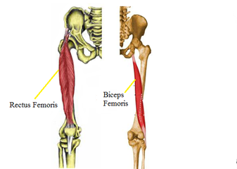Figure 1. Knee joint muscles (Encyclopedia of Science)

2. Literature Review

Human joint muscle behavior is one of the most critical investigations for the orthopedic, biomechanical engineers and researchers. Knee muscles are the complex fibrous structure surrounded by different tissues and blood vanes. The study of muscle behavior has been done by using various methods such as SEMG technique, force analysis by biomechanics or the latest one carried out through FEM technique. Lee et al. developed a 2D FEM knee model for the trans-femoral amputees to estimate the stresses in the muscles. The maximum stresses recorded were 27.4 KPa at the medial side of the adductor Magnus [5]. Tammy et al. developed a 3D model for the knee joint to identify the variables in the selection of meniscal replacement. During FEM analysis three different mesh sizes 1mm, 2mm and 5mm were used. The contact behavior of the knee joint was sensitive to rotational constraints placed on the joint was one of the findings of their study [6]. Blemker et al. developed a 3 D finite element knee and shoulder models for analyzing the behavior of complex muscle. The limitations of the muscle geometry using series of line segment model were overawed by this model. The model accurately predicted the muscle geometry changes till 55° of hip flexion range of motion as compared to magnetic resonance images [7]. Jeffrey et al. described the strategies for 3D FEM modeling of knee ligaments mechanics with a complete joint model and individual ligaments. A novel method to apply in situ strain to FE models of ligaments was proposed [8]. Pena et al. developed a 3D FEM model of knee joint to investigate the maximum principal stress on the knee muscle under anterior and posterior load conditions. Under rotary load condition the role of ligament and menisci in the stability of the knee joint were also investigated [9]. Blemker et al. has developed a 3D FEM model of rectus femoris and Vastus muscle by using magnetic resonance images. By using lumped-parameter models and FEM models the fiber excursions were compared. The rectus femoris complex architecture was studied in detail [10]. Mohsen et al. developed a 3D FEM model of the human buttocks to compute the von Mises stresses during sitting posture. The von Mises stresses developed were in the range of 55 to 65 Kpa [11]. Jiang et al. developed a finite element model to study the sensitivities of tibiomenisco-femoral joint contact behavior in the knee kinematics [12]. Ingrassia et al. worked on a FEM Knee model to analyse the stress and contact pressure peaks between femoral and tibial plates [13]. Chandreshwar et al. developed a statistical shape and alignment modeling (SSAM) approach to characterize the intersubject variability in the knee joint. This study used the relative position of the knee structures through a loaded simulator activity to find the relationship between the variation in shape and relative alignment of the knee joint [14]. Ashutosh et al. has developed a 3D knee joint model to analyze the von Mises stresses at the different load conditions and weights. The 3D model was generated in Pro-Engineer Wildfire 4.0 modeling software. The FEM analysis was done in ANSYS to get the von Mises stresses at different loads. The results predicted that the maximum von Mises stresses were in the range of 1.7MPa to 4.8 MPa acting on the knee joints muscles (upper femur part) when the femur part was fixed and load was applied on the tibial load during flexion leg movement [15]. Adouni et al. computed lower extremity muscle forces and knee joint stresses-strains by using a knee joint FEM model. The results of the model driven by gait data were compared with the data on the normal controls [16]. Lukáš et al. developed a FEM model for hinges PROSPON oncological knee endopprosthesis. The CT scanned knee bones were imported into a CAD model and then FEM analysis of the knee joint during the flexion leg movement was done [17]. John et al. developed a computational knee model to study the influence of hamstrings loading on the patellofemoral pressure distribution. The knee was tested for flexion leg movement from 40° to 80° of ROM. The forces applied during the analysis in rectus femoris was 432N and biceps femoris was 100N during flexion leg movement. During the flexion leg movement the authors have taken the maximum force on rectus femoris than the biceps femoris muscle. The analysis predicted that the rectus femoris muscle takes major stress contribution during the flexion leg movement [25]. Edith et al. developed a knee 3D model to analyse the force and moment generation capacity of the lower limb muscle during walking. During the flexion leg movement, the maximum moment peaked was 13.9 cm in the rectus femoris muscle compared to 11.6 cm in the biceps femoris muscle and also the peak force in rectus femoris muscle was 848.8 N compared to 705 N in biceps femoris muscle in the range of 40° to 70° of the ROM [28].

In the present work FEM analysis of a 3D knee joint is done to investigate the von Mises stresses in two important knee joint muscles; the rectus femoris and biceps femoris muscle during the flexion leg movement. A 3D model is developed for the knee joint muscle analysis by scanning method [11]. During FEM analysis, tetrahedral mesh with 3mm mesh size was used [6]. The maximum von Mises stresses induced during the flexion leg movement were computed. The validation of the results was done by the SEMG test conducted on eight knee prone subjects during flexion leg movements and with the previous researcher’s work [5, 6].

3. Material and Methods

Accurate topology of all the knee bones and muscles is a key to create a valid and accurate 3D knee model, which will be useful for the orthopedic surgeon during pre-operative planning. Therefore, it is logical to base the process of geometrical modeling of the human joints on its anatomical and morphological properties [19].

3.1. Scanning of the Knee Bones

Reverse modeling is one of the fast and accurate option to reproduce a complicated 3D objects such as knee bones. Knee bones modeling in CATIA software without any background help was very difficult and impractical. The irregular shape of the knee bones was difficult to profile in CATIA. By using 3D scanning (ATOS III scanner) four knee bones femur, tibia, and fibula and patella images with the required accuracy and detailed contours were created as shown in Figure 2.

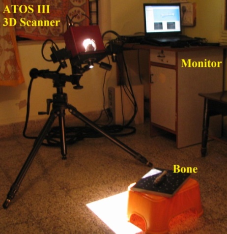Figure 2. Scanning of the tibia by using 3D ATOS III scanner

The scanned object was then imported into geomagic studio. All points outside the relief area were deleted and the various scans were merged into a single data. Thinning of the object was done to reduce total number of points by deleting surplus points in repeatedly scanned areas. Meshing was done to create about 5 million triangles in case of femur. To generate an accurate and detailed model shape-cleaning algorithm was used. Finally .stl file was generated. Similarly the remaining three knee bones (tibia, fibula and patella). stl file was generated.

3.2. CAD Modeling

3D models of bones geometry from scanned .stl file was done in CATIA V5 software. The geometrical features of higher order (curve and surfaces) were designed by filtering and aligning number of cloud points, tessellation of polygonal model, recognition and defining the referential geometrical entities. Complicated contoured 3D model of femur was created by generating anatomical points and spline curves. Similarly tibia, fibula and patella 3D models were designed and detailed contouring was done.

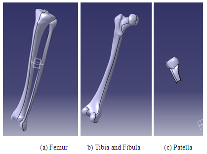Figure 3. Knee bones developed in CATIA V5 model

The mechanical properties of this bone region depend upon the square of the apparent density. According to quadratic dependency, a non-homogeneous bone constitutive law was developed and implemented [20, 21].

Assembly of femur, tibia, fibula and patella in pre-defined direction and coordinates were carried out in CATIA Assembly Design Workbench. The origin, insertion region and careful alignment of the two muscles on femur, tibia, fibula and patella were modeled in CATIA interface. Rectus femoris muscle was modelled on the knee bone from the patella; it is cylindrically shaped at the center, with its width narrowing at the ends and running straight down to the deep apo-neurosis and other end is connected to the hip. Similarly biceps femoris originates from the back side of the fibula and passes obliquely downward and lateral ward across covering the posterior surface of the femur bone to connect on the back end of the hip.

Knee joint contacts and bone muscle contacts were modeled with discontinuous unilateral large sliding laws. It was then imported in .igs format into ANSYS workbench and clean up tool was used for the missing data corrections such as edges and corners. The major difficulty in FEA modeling of knee assembly was to model it to the level where it should mimic the exact motion of the complex knee joint. This is mainly dependent on the surface contact modeling of bones and muscles.

In the present work two types of contacts modeled were bone to bone contact and bone to muscle contact. The model was then exported to ANSYS for the stress analysis. The model comprises three dimensional knee geometry including four major bones and two different knee muscles.

Total 11 surfaces were added in patella to rectus femoris connection, 9 surfaces in rectus femoris to the hip connection, 7 surfaces in tibia to biceps femoris connection and 9 surfaces biceps femoris to hip connection. The important gap between knee joints and axis locations, during flexion were precisely done in the knee CAD model.

3.3. Material Properties

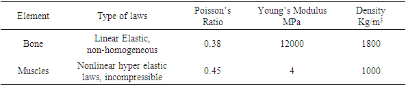
The efficacy of the results obtained in any analysis depends upon its material properties. Sample of all the muscle tissue with various length and thicknesses was used. For rectus femoris and biceps femoris the muscle thickness was taken as 10mm [22]. A non-homogeneous constitutive law was used for bones as well as nonlinear hyper elastic laws were used for rotor cuff muscles and for cartilage. Muscles were considered as an active structure [23]. The muscle element with refined mapped mesh with element size 3mm was used for the analysis. Table 1 explains the different laws and mechanical properties used in knee joint muscle analysis.

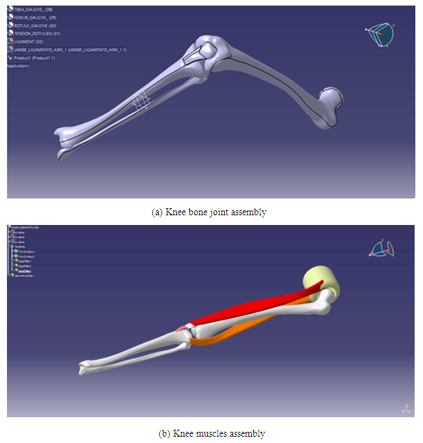Figure 4. Knee joint assembly in CATIA software

Table 1. Different laws and mechanical properties used in the knee joint Model [16, 24, 25]

3.4. Loading Condition

In the flexion, the leg is moved inwards along the single plane of the body. Normal range of motion for flexion of the knee joint is 0° to 120°. Figure.5 shows the flexion and elevation exercise of the knee joint.

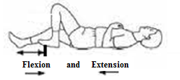Figure 5. Knee flexion and elevation leg movement

The axis of rotation of tibia was tested against the interference with femur, patella and fibula for flexion, from 0° to 120° as shown in Figure 6. Only the self-weight of leg was considered therefore no external weight was added during the FEM analysis. Simulation of the tibia bone with respect to muscles, ligaments and two bones hip and femur was done.

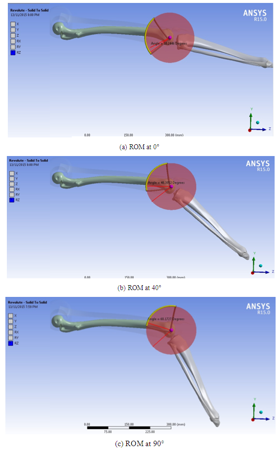Figure 6. Knee joint flexion simulation in ANSYS from 0° to 90° ROM

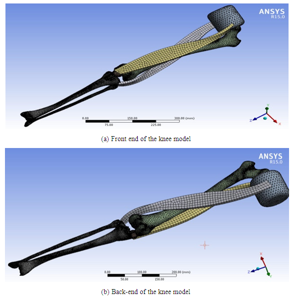Figure 7. Knee joint meshed model with rectus femoris and biceps femoris muscles

3.5. Meshing of the 3D Model

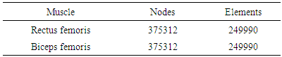
Hexahedral (8 node) and tetrahedral (4 node) 3D solid elements mesh was used in the present model. The quality of the tetrahedral mesh has a profound influence on both the accuracy and efficiency of these simulations. Mapped meshing technique was used to keep the model within quality criteria. After meshing the bones and muscles the number of nodes and elements generated are depicted in the table 2.

Table 2. Summary of number of nodes and elements generated in knee muscle joint FEM analysis

The mesh convergence for knee joint model was done and the knee model has converged to 3mm mesh size for von-Mises stresses. The kinematics for knee flexion was prescribed as an input to finite element simulations. The von Mises stresses of the knee muscles was analyzed for flexion leg movement from 10° to 90° at the interval of 10°. The simulation was done in nine steps in nine seconds and each second corresponds to 10° rotations and the motion was chosen to be pure rotation in a single plane.

4. Results

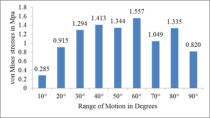
FEM analysis of knee joint muscles for the von Mises stresses during flexion leg movement was done and the results are depicted in Figure 8. As the simulation was done in nine steps at the interval of 10° of rotations, the corresponding von Mises stresses were computed. Probes were added at six different locations in the knee muscles.

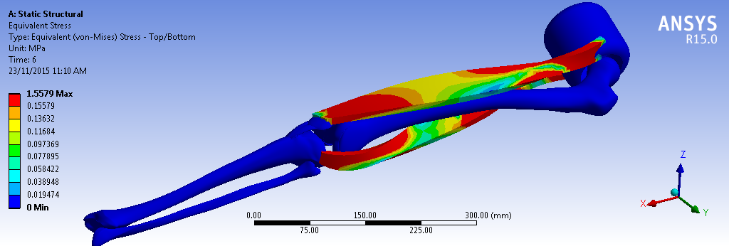Figure 8. Maximum von Mises stresses in rectus femoris muscle

The muscle gets contracted as the knee joint was rotated from 0° to 90° during flexion leg movement. The muscle mass gets broken down and being synthesized with different rates during the leg movements. If the rate of breaking and synthesizing of the muscle mass is maintained (equal) then there will be no stresses induced in the knee muscles. If this rate is not maintained then the net effect will be the tissue formation around the joint and this induces the stresses in the knee muscle. This phenomenon is same for all the muscles in the human body.

Figure 9. Maximum von Mises stresses in rectus femoris muscle

During the flexion leg movement the muscle mass breaking down was more than the synthesizing of the muscle mass and thus the stresses (contraction) were induced in the knee muscles. The muscle mass breaking was maximum in the range of 40° to 70° ROM. [23, 26].

The results predicted that the von Mises stresses had increased from 0° to 60° of ROM and then it declined. The maximum von Mises stresses in the rectus femoris muscle was 1.5579 MPa at 60° ROM during flexion leg movement.

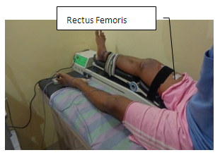
4.1. Muscle Analysis by Surface Electromyography (SEMG)

SEMG was used to study the knee joint muscle behavior of the eight knee prone subjects. The test was conducted during the flexion leg movement on the knee CPM machine for five days. It was conducted under the observation of the Neurophysiotherapist surgeon in Talpallikar Physiotherapy center, Solapur, India.

The maximum knee muscle contraction occurred at the particular angle during the flexion leg movement was observed and plotted. The knee movement was slow and continuous. The motor unit firing amplitudes were observed in rectus femoris and biceps femoris muscles. As the test was conducted during the passive movement of the knee joint muscles, the motor unit firing range was less. Table 3 depicts the motor unit firings in micro volts during the flexion leg movement.

Figure 10. SEMG electrode positions for the knee joint muscle analysis

Table 3. Rectus and biceps femoris contraction during flexion exercise

Figure 11 shows the motor unit firing amplitude variation against ROM one of the subject in the rectus femoris and biceps femoris during SEMG testing on the developed knee CPM machine.

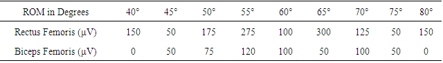
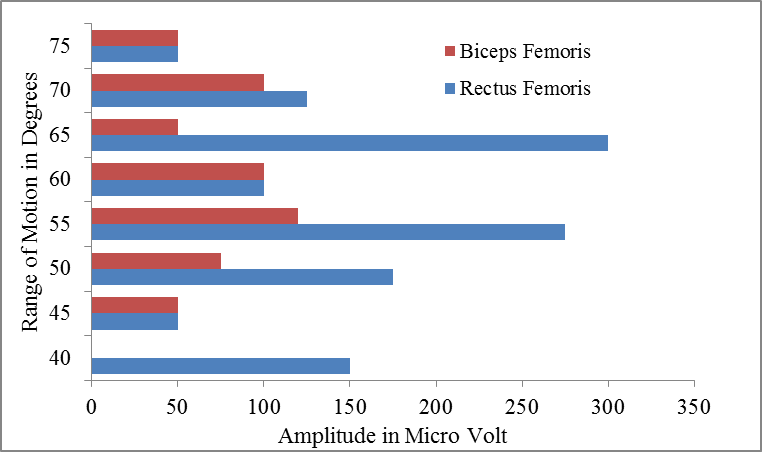Figure 11. Motor unit firing amplitude variation against ROM in rectus femoris and biceps femoris muscles during flexion leg movement

The maximum motor unit firing 300 μV in the rectus femoris muscle was observed from 55° to 65° ROM. The maximum motor unit firing 120 μV in the biceps femoris muscle was observed at 55° ROM.

The same trends were observed in the test conducted on the remaining eight subjects for the rectus femoris and biceps femoris muscles. The SEMG trends showed that maximum contraction during flexion leg movement was in the rectus femoris muscle than the biceps femoris muscle. The maximum motor unit firing during flexion leg movement were observed in the range of 50° to 70°. Thus rectus femoris muscle was the most stressed muscle in the knee joint during flexion leg movement. The same trends were obserevd in the FEM analysis of 3D modeled knee joint. This will help the Orthopeic surgeon to develop and focus on the new therapy to strengthen the rectus femoris muscle during flexion leg movement.

5. Discussion

The purpose of this study was to analyze the stresses induced in different knee joint muscles during flexion leg movement by using FEM model. Accurate and fast 3D knee joint model was generated by reverse modeling technique. ATOS III 3D scanner was used for generating accurate and detailed contours of the knee joint bones. 3D multiple scanning of the bones to obtain a point-cloud model was finalized in the present work. CATIA V5 was used to generate 3D bone from the .stl file imported from the scanned data. Filtering, cloud point alignment, tessellation of the model and referential geometrical entities were done for generating higher order 3D knee bone geometry. According to quadratic dependency, a non-homogeneous bone constitutive law was implemented [20, 21]. Rectus femoris and biceps femoris muscles were added on the knee joint models in CATIA software. The model was imported in .igs format into ANSYS workbench for the von Mises stress analysis. The kinematics for knee flexion leg movements were prescribed as an input to finite element simulations and the resulting muscles stresses were plotted. Muscle initialization and precise location on knee bones were done [7]. In the present FEM analysis there was no clash between knee bone to bone, muscle to muscle and muscle to bone during full range of motion. The muscle thickness varied from 5mm to 15mm along with its length to create a proper volume of tissue over the knee bones. This ensured the real time behaviour of the knee joint with the animated one. During the muscle analysis, the von Mises stresses induced in rectus femoris muscle was maximum (1.5579 MPa) compared to biceps femoris muscle. The maximum von Mises stresses induced was in the range of 50° to 70° flexion angle during the FEM analysis [15, 25, 28].

The present SEMG set up has quantified the muscle behaviour in the knee joint during the flexion leg movement on developed CPM machine. The maximum motor unit 300 μV firing was observed in the rectus femoris muscle at 65° in the probes of SEMG machine during flexion leg movement. The results predicted that muscle contraction for all the subjects during flexion leg movement were maximum in the range of 50° to 70° (average 60°) of the ROM. SEMG analysis has given an indication that rectus femoris was the most contracted (stressed) muscle during the flexion leg movement.

Thus from both the methods (FEM and SEMG) rectus femoris muscle was the most stressed muscle in the knee joint during flexion leg movement. This will help the Orthopeic surgeon to develop and focus on the new therapy to strengthen the rectus femoris muscle during flexion leg movement.

The present work results were in agreement with the work done by [15, 25, 27, 28]. The stress results were also in agreement with the trends of the muscle behavior during SEMG analysis on the eight subjects. The von-Mises stress behavior produced by this FEM model had strong correlations with the actual EMG test done on the patients on the knee CPM machine.

In the present work FEM analysis for knee joint muscle is done for only two major muscles rectus femoris and biceps femoris for flexion leg movement. This work can be further extended by adding Vastus medial, Vastus lateralis Sartorius, semitendinosus, semimembranosus to analyse the von Mises stresses during flexion and extension of leg movement. This will increase the computational cost and degrees of freedom. Due to addition of these muscles the analysis time will increase considerably. In the present work for two muscles FEM analysis took eighteen hours.

6. Conclusions

The purpose of this study was to give researchers and orthopedicians a better understanding about the knee joint mechanism and the most stressed muscle during the flexion leg movements at different ROM. Finite Element Element Method (FEM) analysis was done to investigate the von Mises stresses in two important knee joint muscles; the rectus femoris and biceps femoris muscle during the flexion leg movement. The previous knee models have not considered the stress analysis of the knee muscles during the flexion leg movement. The von Mises stresses from the FEM model has agreed well with the SEMG experimental trends and the previous researchers work in this area. During the 3D FEM muscle analysis rectus femoris muscle was the maximum stressed muscle with 1.5579 MPa compared to the biceps femoris muscle. The muscle analysis for the knee joint was done by using SEMG on eight subjects. The maximum muscle contraction is observed in the rectus femoris muscle in the range of 40° to 70° during flexion leg movement. The same trend was observed in all the eight SEMG tested subjects during flexion leg movements. During the SEMG study; 70% of the muscle contraction was observed in the rectus femoris muscle compared to 30% in the biceps femoris muscle during the flexion leg movement.

ACKNOWLEDGEMENTS

The authors wish to thank Dr. Vyanktesh Metan for validating the data from orthopedic perspective, Dr. Manisha Talpalikar for SEMG analysis and validating trends of the results.