1. Introduction

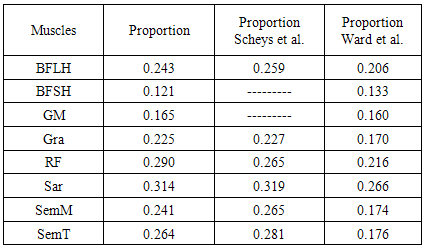
Musculoskeletal models are useful tools to understand the gait of people who suffer a disease that affects their locomotion [1]. Generally, there are two types of musculoskeletal models; Rescaled Generic Models (RGM) and Subject Specific Models (SSM). In today’s clinical practice, the computational tools used for decision making in the treatment of gait problems are based on RGM [2]. Even though RGM have generated important clinical insights, it has been shown that its applicability in the treatment of specific patients is limited due to lack of subject’s specific anatomical knowledge, especially with populations whose anatomy differs from the healthy population. The RGM are generated from the anatomy of healthy subjects with averaged size and weight and then are applied to the patient being studied. On the other hand, the SSM are generated from medical images that represents the own anatomy of the patient being studied; this is why these models have shown better performance in the estimation of biomechanical parameters. For this reason researchers have begun to propose that these models should be the standard method for biomechanical gait analysis in the clinical setting [3].

The muscle paths and its points of origin and insertion are important anthropometric parameters used to calculate muscle moment arm and therefore to understand the mechanical action of muscles around joints. Locations of origin and insertion points are usually derived from anatomic tables [4]. If a model that uses these points is applied to a subject that has some type of anatomical deformation, the biomechanical parameters obtained from the simulation of this model may differ from real values. Scheys et al. [5] has demonstrated that there is a difference between the values of moment arm calculated from RGM and those calculated from SSM for different muscles in people who suffer femoral head deformation due to cerebral palsy.

Muscle paths are generally simplified as a straight line between muscle's origin and insertion points; or a curved line which follows the centroids calculated for the muscles. It has been shown that models that use curved paths estimate moment arm values that are closer to the values measured experimentally [6]. During motion simulation, a modeled muscle can cross into another muscle or bone. To prevent this crossing some clamping surfaces are defined in anatomical structures. These surfaces can be fixed [3], [7], or mobile [6].

Blemker et al. [8] propose a method for creating 3D finite element models of muscle representation, which serve as an alternative to the representation of muscles as straight lines. This representation method tries to solve two limitations presented by the linear models; first the inability of linear models to represent paths of muscles with complex geometry adequately, and second the assumption that moment arms are equivalent for all muscle fibers when actually have different lengths. Although this method increases accuracy of musculoskeletal models, its computational cost remains to be very high, this is the reason why its use in clinical settings remains limited.

A key factor to make possible that parameters such as the origin and insertion points and the muscle paths obtained from SSMs may be used in clinical settings, is to make as efficient as possible the generating process of these models regarding two variables; the time used and the precision with which the structures are rebuilt. These variables depend on the selected image segmentation technique.

In this context, the accurate segmentation of the anatomical structures of interest from medical images determines the efficiency of the SSM. Image segmentation has been traditionally done in 2 ways: one way is to outline manually each structure of interest in each image in the study. These models represent accurately the patient’s anatomy but have poor efficiency due to the large amount of time required to segmenting muscles and bones from the medical images. The other method is to use computer algorithms that perform this process in an automatic or semi-automatic way, reducing processing times and therefore increasing the efficiency of the models. Furthermore these methods allow reproducibility, feature that cannot be achieved with manual methods. Therefore, the goal is to make these computational methods reach anatomical representations comparable to those obtained manually. It is important to note that with exception of the manual segmentation, there is not yet known a universal semi-automatic or automatic segmentation technique that can be used at any application, so up to today it is necessary to adapt the available segmentation techniques to each specific application.

In the field of medical image segmentation, muscles segmentation is a problem that has not yet been fully resolved. The reason is that a basic assumption of image segmentation which asserts that should exist discrimination between the different structures to be identified is infringed. The tissue composition of two different muscles is the same, so if they are closely located it becomes extremely difficult to distinguish one from another [9].

Whitey & Koles [10] identify three generations of medical image segmentation algorithms. The first generation is composed by basic image analysis algorithms such as region growing, edge detection and thresholding. The second generation is composed by algorithms which apply uncertainty models and optimization methods such as statistical algorithms for pattern recognition, deformable models and neural networks. The third generation includes those algorithms that incorporate priori knowledge of the images being processed. Shape models, and atlas based are examples of third generation algorithms.

In recent years, model-based segmentation approaches have been established as one of the most successful methods for image analysis. This techniques match up a model which contains information about the expected shape and appearance of the structure of interest to new images [11]. Nevertheless, these methods uses manual segmentation for creating the models that are going to be deformed to match up the structures in the new images [12], [13].

The goal of this work is to evaluate the performance of a semi-automatic algorithm for segmenting medical images, specifically the interface between muscles. This algorithm allows obtaining from an MRI study, the set of centroids which represent the path of a given muscle from its origin to its insertion point, reducing the processing time while retaining high levels of sensitivity and specificity.

2. Methodology

This paper presents a semi-automatic segmentation algorithm based on Dijkstra's shortest path algorithm. In this section the algorithm developed using Matlab®, and the tests executed are presented.

2.1. The Shortest Path Algorithm

In 1959 Edsger Dijkstra proposed an algorithm to solve two fundamental problems in graph theory: the problem of minimum weighted spanning tree and the shortest path [14]. From this publication onwards Dijkstra’s algorithm for obtaining the shortest path between two points has become one of the most outstanding algorithms in computer science. It is mainly used in vehicle routing planning devices to find the best route between two locations [15, 16].

A digital image can be seen as a graph where its vertices are each of the image pixels and the paths restrictions can be understood as the difference between the grey level of a pixel v1 and the level of another pixel v2 in the image. It can also be assumed that the pixels that make up an object within an image have homogeneity between grey level values, and that are different from the surrounding background. In this framework it is possible to design a segmentation algorithm that properly differentiates bones and muscles and even the boundary between closely located muscles.

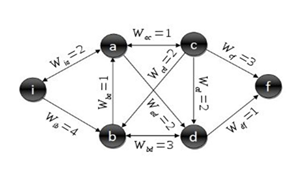Figure 1. Standard graph for shortest path calculation

For the graph shown in Figure 1, the shortest path between vertex i and vertex f is calculated taking into account the existing restrictions to passage from a vertex v1 to another one v2. The steps to calculate the Dijkstra’s shortest path between these vertices are described by [17]:

1. Choose the source vertex.

2. Define a set S of vertices, and initialize it to empty set. As the algorithm progresses, the set S will store those vertices to which a shortest path has been found.

3. Label the source vertex with 0, and insert it into S.

4. Consider each vertex not included in S connected by an edge from a previous vertex to a newly inserted vertex. Label the vertex not in S with the label of the newly inserted vertex, for which the cumulative weight is calculated from the initial pixel up to the previous vertex with which it is connected plus the weight of the edge of the previous vertex and the new vertex. (But if the vertex not in S was already labelled, its new label will be the minimum weight of the paths between the initial vertex and the newly inserted vertex).

5. Pick a vertex not included in S whose sum of weights from the initial vertex was the one with the minimum value, as a result this new vertex is inserted in S.

6. Repeat from step 4, until the destination vertex f is included in S. In this way the problem of the shortest path is solved or until there are no more vertices that could be labeled. In this case the minimum path was not found. If the destination vertex is labeled, its label is the distance from its position and the source i. If it is not labeled, there is no path from the source vertex i and the destination f. This last situation is not expected to happen in the image segmentation algorithm proposed in this work, because there is always a connecting path between any two pixels in an image.

The developed shortest path algorithm has as output the closed region obtained by applying the Dijkstra’s algorithm above described, between a set of pixels selected as belonging to the edge of the structure wanted to be segmented. These points are selected by a medical expert and are known as seed points.

As initial step the algorithm takes the first selected seed pixel, and from this pixel, sorts the rest seed pixels on clockwise direction. Initial vertex is defined as the first pixel in the sorted list and final vertex as the second pixel in the same list. Dijkstra’s algorithm is applied between these two pixels, thereby obtaining the first portion of the segmented region. Then, the new initial vertex is defined as the final vertex at the previous step and the new final vertex as the next pixel located in the sorted pixels list. This procedure is repeated until the algorithm detects that the Dijkstra’s algorithm was applied between the penultimate and the last pixel in the sorted pixel list; then it defines as initial vertex the last pixel in the sorted list and as final vertex the first pixel in the sorted list and applied one last time the Dijkstra’s algorithm between these two vertices. When the whole closed region is extracted, the algorithm computes the geometric centroid by the areas method and stores that value together with the region information obtained.

Dijkstra algorithm has a computational complexity of . In the worst case scenario n((n-1))⁄2 sums and n(n-1) comparisons are performed. In the analysis of big graphs, this complexity involves the use of large amount of memory this is the reason why computational performance of the algorithm is considerably low. This is why several improvements to the original algorithm has been continuously proposed [17, 18]. This problem affects the proposed algorithm as the images on which it works have a size of 512x512 pixels, this was checked in the early versions of the algorithm where the average segmentation time to each muscle or bone in one slice was around 35 minutes. For this reason for each pair of initial and final vertices defined during the segmentation process described above, the last version of the algorithm performed an automatic sub-sampling of the image applying Dijkstra’s algorithm on this sub-image and not on the complete image. This sub-image is defined as a rectangular region whose corners were located at a distance of 10 pixels to the outside of each pair of pixels defined as initial and final vertices. With this distance, the algorithm is able to improve its performance considerably without losing quality in the segmentation results due to a loss of information related to sub sampling the image.

2.2. Executed Tests

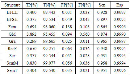
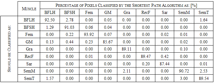
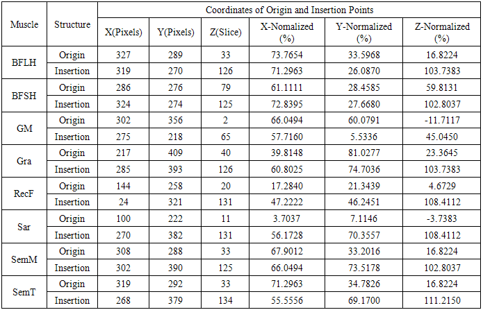
The main image acquisition techniques used in the development process of musculoskeletal models are: Magnetic Resonance Imaging (MRI) and Computed Tomography (CT). Numerous studies have been conducted using both techniques [3, 19-21]. MRI allows acquiring images of muscles, bones and cartilage simultaneously with high spatial resolution; it also has the capacity of multiplanar acquisition and does not produce ionizing radiations, as CT does. For this reason in this paper MRI is used as the imaging acquisition technique. A set of 136 MR images from a healthy subject were obtained using a T1-weighted-spin-echo sequence (TR=400ms, TE=17ms, Matrix=512x512, FOV=25cm, Gap=4mm) on a 1.5 T device Siemens Magnetom Vision. The tested subject signed an informed consent. Prior to images acquisition a set of small soy spheres which served as external markers of anatomical structures was placed on the subject's skin using hypoallergenic tape. The marked anatomical structures were Antero Superior Iliac Spine (ASIS), the Spinous Process of the fifth Lumbar Vertebra (LV), and the lateral femoral condyle (LFC). These markers are used because they are an anatomical point of easy external location and therefore can be used to make comparisons between different subjects and develop SSMs. With these markers a coordinate system whose origin is located at the centroid of the marker in the ASIS was defined.

The femur bone (Fem), and the muscles; Sartorius (Sar), Rectus Femoris (RecF), Gracilis (Gra), Biceps Femoris Long Head (BFLH), Biceps Femoris Short Head (BFSH) Semitendinosus (SemT), Semimembranosus (SemM) and Gluteus Maximus (GM) were segmented. The segmentation was performed in two ways. Firstly it was manually performed by a medical expert, and secondly using the shortest paths algorithm. For the application of the latter algorithm the expert was asked to place no more than 15 seed pixels per muscle or bone segments. The regions obtained by manual segmentation are considered the gold standard.

After performing segmentation of the complete set of images, each subgroup of origin and insertion regions of each muscle was taken, and then an average coordinate which serves as an "effective" point of contact between muscle and bone was calculated. However the real contact area can also be defined, and then proceeds to calculate standardization system coordinates mentioned above and described below. To each external marker his centroid was calculated and a coordinate axes system was defined. With this system for the different segmented muscles, the location of each "effective" origins and insertions points were referenced. This location was normalized in respect to the magnitude of the vector connecting the centroids of the different external markers. These distances correspond to the normalized magnitude of the projection on the X axis of the vector joining the centroids of the markers in the IPM and in the AE for the X component, the magnitude of the projection on the Y axis of the vector joining centroids of the markers in the IPM and in the AE for the Y component, and the magnitude of the vector joining the markers in the IPM and the CLF for the component Z. This means that the location of the patient on the stretcher was in rest horizontal position.

With origin and insertion points, muscle-tendon length was calculated for each muscle, this was done by calculating the Euclidean distance between the point of origin and the insertion.

As indicators of the segmentation quality obtained by the algorithm the values of Sensitivity (Sen) and Specificity (Spe) were calculated. The calculated value of Sen measures the ability of the algorithm to identify pixels that actually belong to the segmented structure. And the calculated value of Spe measures the ability of the algorithm to identify pixels that do not really belong to the segmented structure, according to:

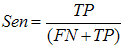(1)

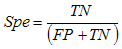(2)

Where TP is the True Positive pixels value, i.e. the number of pixels that both the manual segmentation and the semi-automatic algorithm defined as belonging to the segmented region; TN is the True Negatives pixels value, i.e. the number of pixels that both the manual segmentation and the semi-automatic algorithm defined as non-belonging to the segmented region; FP is False Positive pixels value, i.e. the number of pixels that manual segmentation defined as non-belonging to the segmented region but the semi-automatic algorithm defined as belonging; and FN is the False Negatives pixels value , i.e. the number of pixels that manual segmentation defined as belonging to the segmented region but the semi-automatic algorithm defined as not belonging.

Another indicator of the segmentation quality of the algorithm proposed is the confusion matrix. This matrix is obtained taking the pixels of the segmented region by the proposed algorithm for each structure comparing if these pixels were classified by the gold standard as belonging to those structures or to different ones. The confusion matrix has as evaluation method the advantage that is not affected by the major or minor proportion that has the structures to be segmented compared respect to the size of the image. This factor is important if the size of the muscles of the images taken in this work from the muscles and bones are inferior compared to the total size of the images. In addition, it allows the identification of the capacity of the algorithm to differentiate structures that are closely located.

3. Results and Discussions

Manual segmentation by medical expert and segmentation with the shortest path algorithm were performed, for each of the eight muscles and bone, in the 136 images acquired in the MRI study. As an example a section of each of the segmented structures is shown in Figure 2.

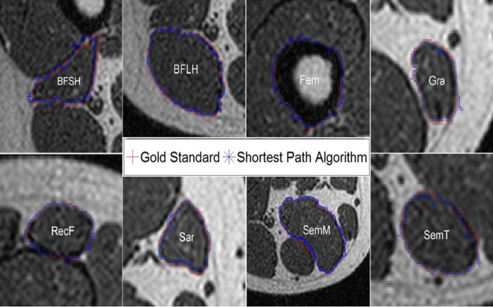Figure 2. Segmented regions obtained from the group of images by means of the semi-automatic algorithm for each muscle and femur bone

Table 1 contains the values of Sen and Spe obtained for each muscle and the femur. As can be seen, the values of Sen in all cases are above 90%, these values are indicative of the ability of the algorithm to correctly identify the structure being segmented. The Spe values close to 1 obtained for all structures are due to the difference in size between different segmented structures and the total image size. These high values of Spe were expected because the algorithm performs the segmentation using the seed points selected by the medical expert.

Table 1. Sensitivity and Specificity Values for each Segmented Muscle

Table 2 shows the confusion matrix calculated for the segmentation of the entire group of structures. The results contained in this table account for the ability of the developed algorithm to clearly differentiate between two closely located structures. For example it can be seen that the algorithm correctly classified 89.54% of the pixels belonging to SemT muscle, and 90.72% of the pixels belonging to SemM muscle. These two muscles are difficult to identify because they are closely located. However, it can be seen that the algorithm fails to classify only 3% of pixels as belonging to the SemT muscle when actually belong to the SemM muscle, and also fails to classify only 2.53% of pixels as belonging to the SemM muscle when really belonged to the SemT muscle.

Table 2. Segmentation Confusion Matrix

The position of actual points of origin and insertion for each of the 8 segmented muscles was calculated with the data obtained from the segmentation of the entire group of images.

Figure 3 shows as an example how the ''effective'' origin point of the BFSH muscle was calculated, in the same manner the ''effective'' origin and insertion points of the remaining muscles were extracted. The "effective" areas of origin and insertion were calculated as the average of the contours in the contact between muscle and bone in each image.

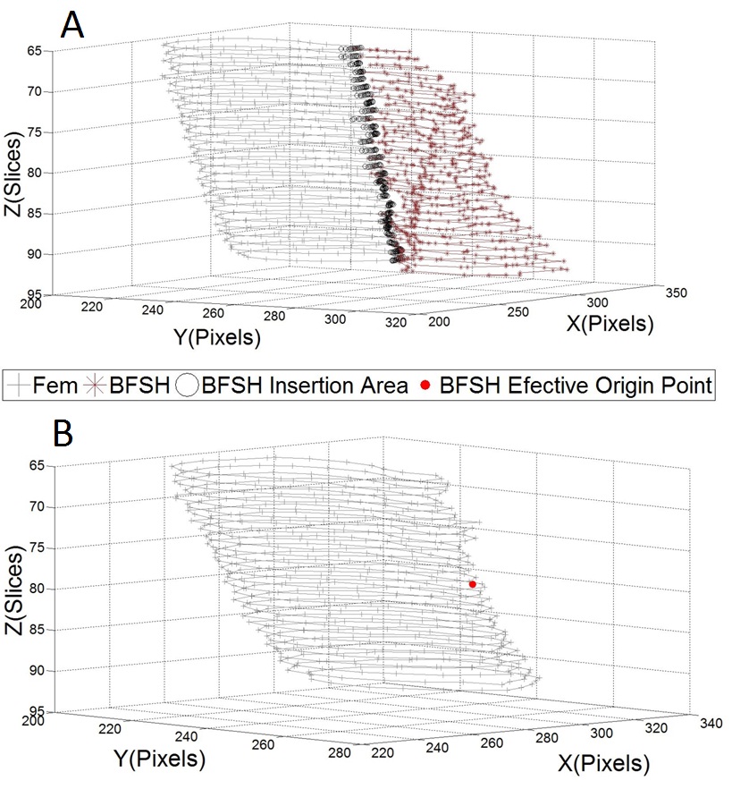Figure 3. Effective origin point calculation of the BFSH. The + symbols refers to the Fem borders. The * symbol refers to the BFSH borders. The o symbols refers to the contact area between Fem and BFSH. The symbol • refers to the calculated BFSH ''effective'' origin point, calculated as an average of the contact area for each of the slices of the previous regions

Table 3 shows coordinates (X, Y) in pixels and the image number (representing the Z coordinate) where each "effective" origin and insertion points are located for each segmented muscle. Also, in this table the locations of these points are shown relative to the standardized coordinate system (see Methodology). The use of the alternative coordinate system and the standardization with respect to the magnitudes of the vectors connecting the external markers used here allows on future works to make comparisons between the results obtained for different subjects and generate anthropometric dimensionless tables of a healthy population or a population with a defined anatomical deformation. This is because the ASIS, the AE and the CLF are external anatomical markers usually used in clinical biomechanics laboratory and can be easily located.

Table 3. Muscle's effective Attachments Sites

The muscle-tendon lengths for each muscle were calculated with the data contained in Table 3, these results can be seen in Figure 4. Furthermore, the muscle-tendon lengths presented by Scheys et al. [3] and those reported by Ward et al. [22] for the same muscles are shown in this figure. The difference observed between lengths is because the data are not normalized to the heights of the tested subjects. These heights are 153 cm in this work, 185 cm in the work of Scheys et al. [3], and 168 cm in the work of Ward et al. [22]. However, from the lengths shown in Figure 4 can be seen that the ratio between the lengths of the muscles on each subject are very similar.

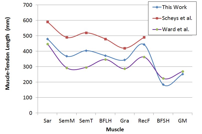Figure 4. Calculated muscle-tendon lengths (mm) for each muscle: in this work from the calculated "effective" origin and insertion points, and the muscle-tendon lengths reported by Scheys et al [3], and by Ward et al [22]

Specifically, the data is not normalized in this figure because they give a better idea of proportionality between the different estimation methods. The matching estimates between this article and the other works can be seen in the data reported in Table 4. In this table the ratio between length of each muscle and height of the subject were calculated.

Table 4. Muscle-Tendon Lengths / Height Ratios

Figure 5 shows the centroid path calculated for all segmented muscles. This figure also shows some bone structures that allows a better visualization of the muscle's path. With the 3D locations of the centroids could be possible to generate a mathematical function that fits these muscular paths. This mathematical description could be used to calculate more accurately the torque applied by each muscle on the joints where it crosses.

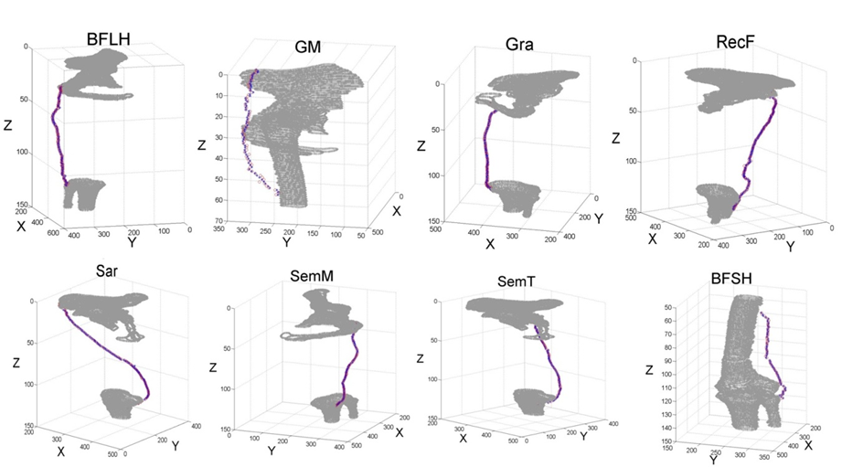Figure 5. Centroid paths obtained with manual segmentation (+) and with the shortest path algorithm (*) for each muscle

4. Conclusions

This paper presents a second generation semi-automatic segmentation algorithm based on the Dijkstra’s shortest path algorithm to obtain origin and insertion points, and muscle paths from medical images. This algorithm significantly reduces the processing time while retaining high levels of sensitivity and specificity on the segmented structures. These characteristics make it a good choice for both the formation of SSMs, and the formation of anthropometric parameters databases sufficiently precise that can be used in simulating RGM.

In the continuation of this work, it is expected that the shortest path algorithm proposed in this paper can be used as training algorithm of a pattern recognition system that reduces the time required for the segmentation of an MRI study. In this sense it could be achieved the generation of the initial statistical patterns that can be deformed to a final segmented region and after this process the generation of SSM and more efficient and accurate RGM that can better represent the results obtained experimentally in a laboratory of biomechanics.

ACKNOWLEDGEMENTS

The authors would like to thank to National Council of Scientific and Technical Research (CONICET) and the research project PICTO 222-2009 to provide the funds needed for this research. Also the authors would like to thank to prof. Claudia Schira for her valuable collaboration.