1. Introduction

For contrast imaging of blood flow, the quantity of microbubbles changes in the perfusion region of interest and generally the microbubbles have a time varying size distribution. From size distribution measurements, it can be seen that there is a substantial decrease in mean bubble size and in volume fraction of agent with increasing flotation times [1, 2]. Soetanto and Chan measured the size distributions of microbubbles and observed that the distributions were nearly normal distributions and shifted gradually to small sizes over time [3]. Hoff also obtained the similar results, where size distributions were measured by the Coulter Multisizer [4] after varying flotation times.

The time varying size property of microbubble will make harmonic images time varying and frequency sensitive. Krishna and Newhouse measured the characteristics of harmonics of different contrast agents and found that the first harmonic decayed more rapidly with time than the second harmonic [5]. Shi and Forsberg showed the amplitudes of the harmonics are time-dependent and quite different for 2-MHz insonification compared to 4-MHz insonification [6].

Since bubble echo depends greatly on resonance, which is size and frequency dependent; therefore optimal transmission frequency (TxF) selection is essential to maximize the backscatter power of microbubbles for contrasting imaging to increase SNR. Toilliez et al. [7] and Wyczalkowski [8] et al. proposed optimal techniques to enhance bubble scattering and maximized bubble translation. Reddy and Szeri focused on optimizing the driving pulse to exploit the transient response for pulse-inversion imaging [9]. Menigot et al. suggests Gradient ascent method to find the optimal frequency adapted to microbubble [10]. Kaya et al. assessed the acoustic response of lipid-encapsulated monodisperse microbubbles in response to different excitation frequencies. They investigated means to achieve optimal acoustic response based on the relationship between resonant frequency of microbubbles and center frequency used for transmission [11]. Moon et al. measured microbubble echo signals at various frequencies. They found driving a specific frequency in harmonic mode is capable of maximally resonating micrbubbles with a narrow size distribution could enhanced ultrasound imaging [12].

Optimal TxF can be found using simulating echo responses based on bubble oscillation model, whose results were shown to be in a good agreement with experimentally measured echoes [11]. For this method, each TxF must be considered as input of the simulation model and it costs much time to solve the Raleigh-Plesset equation.

In this paper, we propose a theoretical method to search the optimal TxF, which yields maximal power for harmonic chirp imaging [13] and does not need to solve the Raleigh-Plesset equation. This method is based on the scattering cross-section of microbubble given by Church [14] to model the bubble harmonic backscatter power for chirp excitation. In this way, the second harmonic backscatter power can be derived as a function of the second harmonic scattering cross-section, bubble size distribution and square of the transmission signal, which is a function of the TxF. Then the optimal TxF can be taken to be the frequency that can yield maximal power among all possible frequencies. For convenience, this method is named SCS (Scattering Cross-Section) method.

In the follows, the theories for required computations are given in section II. Definitions of the SCS method is given fist. For comparison, a method for optimal TxF selection using simulation signals is presented next. In order to verify the SCS method, the improvement factor predicted by the SCS method is compared with that predicted by simulation signals generated by BubbleSim [15] in section III. Some properties of the optimal TxF found by SCS method are presented in section IV. For convenience, the equations of [14] used in this study are digested and put in the appendix.

2. Theories

2.1. Optimal TxF Selection Based on SCS

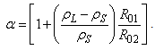
Based on Church’s formulation [14], for a microbubble coated with an elastic solid shell, its second-harmonic SCS can found to be a function of driving frequency, f, as, where r is the radius of microbubble. For convenience, the equations of [14] used in this study are digested and put in the appendix. They include the resonant frequency (A.1) and scattering cross-sections of first and second harmonics (A.2 and A.3).

For a mixture of bubbles with size density , its second-harmonic SCS can be expressed as sum of the individual second-harmonic SCS's of bubbles with different sizes as:

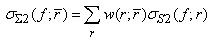(1)

where is the mean bubble size, and is named TSCS (Total Scattering Cross-Section). Since is an analytic solution of the RPNNP bubble equation, its value can be computed easily.

In this study, the bubble size density, , is assumed to have a Gaussian distribution with being the mean bubble size and the standard deviation being [1, 4]. Since the Gaussian function is an unimodal function, the TSCS is an unimodal function of driving frequency also. This ensure that, for a given bubble size distribution, there is an unique optimal driving frequency , which can be found as

(2)

This is the SCS method for finding the optimal driving frequency for a mixture of bubbles.

2.2. Optimal TxF Selection Based on BubbleSim Signals

BubbleSim is a simulation program developed by Hoff for solving the nonlinear bubble equation to get the bubble echo signal for a given driving signal [15]. Unlike the SCS of bubble, the result of BubbleSim can provide much detail information about the bubble echo. This includes the effects of amplitude, frequency, waveform of the driving signal and other bubble characteristic parameters. 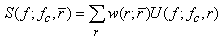For the convenience in specifying the harmonics of the bubble signal with different bubble size, the driving and bubble signals will be denoted as and when necessary, where is the center frequency of the driving signal and r is the bubble radius.

As in the SCS method, the total power of the second harmonic of bubble echo can be found as

(3)

where is the second-harmonic power (SHP) of a bubble with radius r. One way to find the SHP is to use the pulse inversion technique [15, 17], which needs to transmit two phase-inverted driving signals to find the second harmonic, , of . By Fourier transform, the power spectrum of the second harmonic can be found to be

(4)

Then the SHP can be found to be

(5)

where is the twice of TxF and is bandwidth of driving signal.

As in the SCS method, the optimal driving frequency, , can be found as

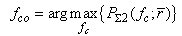(6)

This is the BubbleSim method to find the optimal driving frequency for a mixture of bubbles. It is noted that, to find the total second harmonic power, , the bubble equation must be solved for different bubble sizes, which is very time consuming. Even more serious is that the total second harmonic power must be computed for different driving frequencies to find the optimal driving frequency, . This will be prohibitive for practical usage.

3. Simulation Studies

3.1. The Use of SCS Method

For demonstrating the SCS method, the TSCS's of three different mixtures of bubbles are computed for optimal TxF selection. The mean bubble sizes used are 2, 1.5 and 1 μm and the standard deviation of bubble size is set by . For each bubble, the SCS of second harmonic are computed using Eq. A.3 with the following settings:

Shell thickness = 4 nm, Shell shear modulus = 50 MPa, Shell viscosity = 0.8 Pas, Ambient pressure = 100 KPa, Polytropic exponent = 1, Viscosity of the liquid = 0.001 Pas, Density of the surrounding liquid = 1000 kg/m³ and Density of the shell material = 1100.

Three TSCS's are shown in Fig. 1. In each figure, the values of TSCS at two TxF's are given and marked with dashed arrows. One is the optimal TxF and the other is 2.25 MHz for comparison. The TSCS of a TxF is represented as P(TxF); for example, in Fig. 1-a, "P(1.70 MHz) = - 96.4 dB" means that the TSCS at f_co=1.70MHz is - 96.4 dB. The TxF, 2.25MHz, is chosen to be a reference case for showing the performance of the optimal TxF and it represents a non-adaptive situation that use a fixed TxF, f₀=2.25MHz, despite of the change of bubble size. In dB scale, the difference, , is the improvement factor (IF) of the optimal TxF relative to the reference TxF, . For the three types of bubble mixture, the improvement factors of using the optimal TxF are 2.5, 0.3 and 7.4 dB.

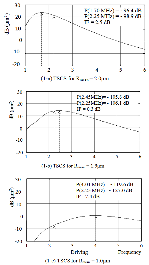Figure 1. The TSCS of second harmonic for three types of bubble mixtures

3.2. Verification of the SCS Method by BubbleSim

Although the proposed SCS method can find an optimal TxF for a given bubble mixture without solving the bubble equation, its result has nothing to do with the driving signal. In imaging applications, the driving signal is pulsed and bandlimitted, which may have complicated effects on bubble echo due to the nonlinearity of bubble. However this is not a problem for the BubbleSim method, since BubbleSim solves the bubble response for a given driving signal. To verify the usefulness of the optimal TxF predicted by the SCS method, the IF's of the optimal TxF's shown in last section are examined using BubbleSim method.

The power of bubble responses to a chirp signal driving at the optimal TxF are found by BubbleSim for comparison with that of the non-adaptive case. The chirp signal is set to have bandwidth = 1 MHz and transmission acoustic pressure = 50 KPa, and is shaped by a Hanning window to have pulse length = 10 μs. In BubbleSim, the bubbles are simulated using the modified Raleigh-Plesset equation with parameters set as in [15]: Shell thickness = 4 nm, Shear modulus = 50 MPa and Shear viscosity = 0.8 Ns/m².

The simulation results are presented using the PSD (Power Spectral Density) of bubble echoes. The PSD of the echoes of a bubble mixture is defined as:

(7)

where is the power spectrum of the second harmonic of bubble echo as defined in (4). The second harmonic of bubble echo is extracted by the pulse inversion technique and is the bubble density.

The PSD's of the same bubble mixtures defined in last section are shown in Fig. 2. In each figure, two PSD's are given, one is for the optimal TxF predicted by the SCS method and the other is for the reference frequency f₀= 2.25 MHz. For example, in Fig. 2-a, the black one is the PSD of the second harmonics of the bubbles with mean size = 2 μm driven by the optimal TxF and the blue one is that driven by the reference frequency. Since they are PSD's of simulation signals, they are affected by non-suppressed harmonics. For the black one, its main response is located at 3.4 MHz, which is the second harmonic of TxF = 1.7 MHz, and the other response at 6.8 MHz is the fourth harmonic. Similar results can be found for the reference case. Based on the PSD's, the IF can be found to be 1.3 dB for the 2 μm bubble mixture. For the other two type of bubble mixtures, the improvement factors are 0.2 and 4.3 dB.

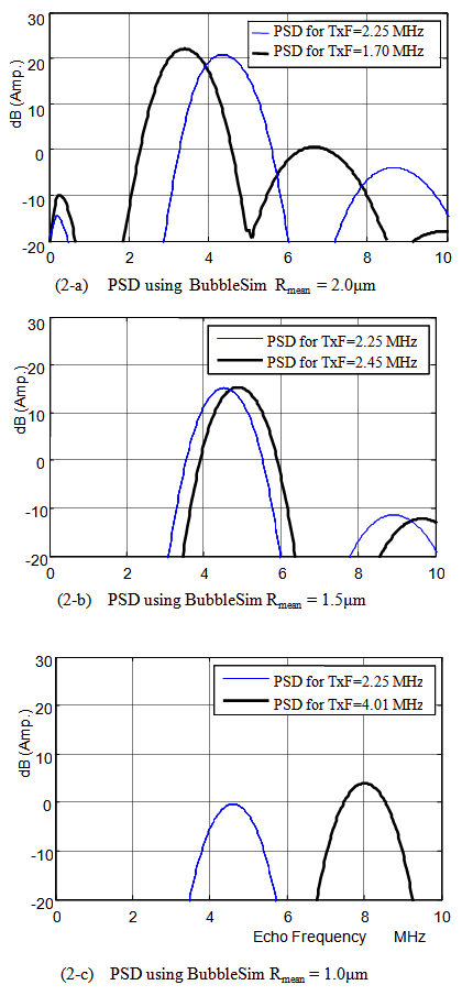Figure 2. The PSD of second harmonic for three types of bubble mixtures

Comparing the above results to the SCS method given in Sec. III-A, the following observations can be found. For the three types of bubble mixture, the IF's predicted by the SCS method are 2.5, 0.3 and 7.4 dB and the IF's predicted by the BubbleSim method are 1.3, 0.2 and 4.3 dB, which are all smaller than those predicted by the SCS method. Although the IF's predicted by SCS method may be too promising, the optimal TxF's predicted by SCS method do yield power improvements as verified by BubbleSim.

There are two major reasons that make the simulation results different from the predictions by SCS method. (1) By definition, SCS is the intensity gain of a bubble excited by infinite long sinusoidals, which is different from the pulsed signal used in BubbleSim. (2) The SCS given in [14] was derived based on the analytical solution of the RPNNP bubble equation, which is an approximate solution under weakly nonlinear assumption. This assumption is not required in BubbleSim. Therefore the results of BubbleSim are not so restricted as those of SCS method.

For further verification, the IF's of SCS method are examined for 8 different bubble densities with mean bubble size being decreased from 3μm to 0.4μm as: 3μm, 2.5μm, 2.0μm, 1.5μm, 1.0μm, 0.8μm, 0.6μm and 0.4μm. The corresponding optimal TxF's predicted by the SCS method are 1.02MHz, 1.28 MHz, 1.7MHz, 2.45 MHz, 4.01 MHz, 5.19 MHz, 7.19 MHz and 11.57 MHz. As above, the reference one uses f₀=2.25MHz for all 8 cases to predict the IF's of the optimal TxF's. Then the IF's of the optimal TxF's are evaluated by BubbleSim using the same setting as before. The IF's are shown in Fig. 3.

Comparing the optimal TxF's with the reference frequency, it can be found that:

1) The 1.5μm bubble mixture (optimal TxF = 2.45MHz) is the one that closest to the reference case (Txf = 2.25MHz).

2) The optimal TxF's increase as mean bubble sizes decrease.

3) The change of optimal TxF's increase as the mean bubble sizes decrease, especially when it crosses the reference case; this means that the sensitivity of TxF's to bubble size is higher for small bubbles than for large bubbles.

Comparing the IF’s for different cases, it can be found that:

1) The sensitivity of IF to TxF is higher for large bubbles (on the LHS of Fig. 3) than for small bubbles (on the RHS of Fig. 3). This property is a consequence of the scattering property of bubble, which can be confirmed by comparing the TSCS’s given in Fig. 1. The shape of the TSCS around , given in Fig. 1-a, is sharper than those given in Fig. 1-b and 1-c; this means that the TSCS of large bubble is more sensitive to TxF than that of small bubble.

2) A general property of the IF’s is that IF increases monotonically as the distance between the optimal and reference frequencies, i.e., , increases.

3) The IF’s predicted by the SCS method is in general larger than those predicted by BubbleSim. However, since these two predicted IF’s are proportional to each other, this is enough to confirm that the SCS method is a proper technique for optimal frequency selection for varying bubble size distribution.

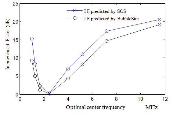Figure 3. Improvement factor verification for different mean bubble sizes: 3.0μm ~ 0.4μm

4. Properties of the Optimal TxF

The reason that bubble echo intensity can be optimized by TxF is due to the resonant property of bubbles. For a bubble mixture of different sizes, which is known as poly-dispersive bubbles, the bubbles are excited to different degree of resonances; its optimal TxF depends on the mean size as well as the size spread of the mixture. To see the effect of bubble-size spread on the optimal TxF, the optimal TxFs for three types of bubble mixtures are found, using the same parameter setting as in section III.A, and plotted in Fig. 4. The mean bubble size () is varied from 0.5 to 5μm and the standard deviation of bubble-size is set by , with c =0,0.1 and 0.3.

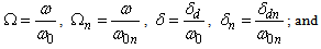
When , it is the case of mono-dispersive bubble, i.e., single-sized bubble. The optimal TxF for a bubble with radius is defined by its SCS at its resonant frequency, i.e., , where is the resonant frequency. This is the simplest case that the optimal TxF is just the resonant frequency, which is the red curve in Fig.4 computed using Eq. A.1. In general, the resonance frequency of bubble is inversely proportional to bubble size. This property can not be observed easily based on the resonant frequency given by Eq. A.1, since it is not a simple function of bubble size. However, based on other formulations, such as the resonant frequencies given in [4] and [18], the resonant frequency of microbubbles can be approximated as a function of . When bubble particle is described by its bulk modulus , its resonance frequency can be expressed in a simple form as given by Minnaert

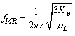(8)

where is the density of surrounding liquid.

Apparently, the optimal TxFs of poly-dispersive bubble cloud (green and blue) follow the trend of the resonance frequency of single-sized bubbles. This shows that the resonance frequency and SCS of mono-dispersive bubbles is useful for inferring the optimal TxF of poly-dispersive bubble cloud. In general, The resonant frequency increase as mean bubble sizes decrease, so is the optimal TxF. As the property of resonant frequency, it can be said that the optimal TxF is roughly proportional to , if the size spread is small. In addition, Fig. 4 shows that the optimal TxF of a poly-dispersive bubble cloud with size distribution parameters is lower than the resonance frequency of single-sized bubble with . The larger the is, the lower the optimal TxF is. This is due to that bubble power can be maximized by reducing TxF to excite larger bubbles to resonant when is large.

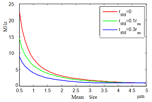Figure 4. Optimal TxF for different size spread

As done in the comparison study of last section, by observing the three TSCSs given in Fig.1, it can be found that a general property of the TSCS of second harmonic is that the TSCS of large bubble has small spread (or width) and vise versa. The width of TSCS can be defined as the resonant-bandwidth (RBW) of TSCS. In principle, smaller RBW means that the IF of bubble echo power is more sensitive to TxF. To further exploit this property, the RBW of the SCS of mono-dispersive bubbles are computed and plotted in Fig.5 (red) along with the resonant frequency (blue). It is found that the RBW of the SCS follows the trend of resonant frequency. Large bubble has small resonant frequency as well as small RBW; this confirms that the IF of large bubble is more sensitive to the use of optimal TxF than that of small bubble. In other words, the power sensitivity of large bubble is higher than that of small bubble. This property sets a conclusion that the use of optimal TxF is more important for large bubble than for small bubble.

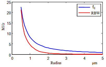Figure 5. Resonant frequency and bandwidth (RBW) for bubbles with different size

5. Conclusions

For optimizing the SNR in contrast imaging, an analytical technique, named SCS method, for optimal transmission frequency selection is proposed. The correctness of the SCS method is validated using simulation signals generated by BubbleSim.

Based on results of the test cases, it is found that the sensitivity of TxF's to bubble size is higher for small bubbles than for large bubbles; however, the sensitivity of IF to TxF is higher for large bubbles than for the small bubbles. Based on the RBW of SCS, it is concluded that the use of optimal TxF is more important for large bubble than for small bubble.

Since the SCS method is an analytical technique, it is computationally efficient and can be the basis for developing an adaptive TxF selection technique. However, it needs the knowledge about bubble size distribution. To be an adaptive technique, bubble size distribution must be estimated in time. This calls for a technique to estimate the time-varying bubble size distribution based on bubble echoes.

ACKNOWLEDGEMENTS

This work is supported by the National Science Council, Taiwan, NSC 102-2221-E-002 -024.

Appendix

The resonant frequency and scattering cross-section of microbubble digested from [14] are given below. The linear resonant frequency can be predicted by:

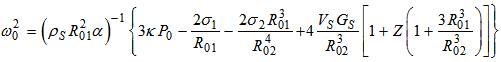(A.1)

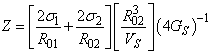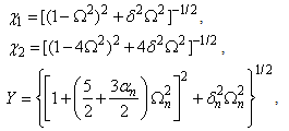
with and .

The scattering cross-section for the first and second harmonics of a bubble coated with an elastic solid and driven by of an incident frequency of are predicted to be

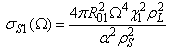(A.2)

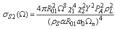(A.3)

where