1. Introduction

The analysis of the electrocardiogram as a diagnostic tool is a relatively old field and it is therefore often assumed that the ECG is a simple signal that has been fully explored. However, there remain difficult problems in this field that are being incrementally solved with advances in techniques from the fields of filtering, pattern recognition, and classification, together with the leaps in computational power and memory capacity that have occurred over the last couple of decades. While the ECG is routinely used to diagnose arrhythmias, it reflects an integrated signal and cannot provide information on the micro-spatial scales of cells and ionic channels. For this reason, the field of computational cardiac modeling and simulation has grown over the last decade. The aim of this paper is by using a novel system to develop methods to analyse and detect small changes in ECG waves and complexes that indicate cardiac diseases and disorders. ECGs are normally displayed with 25 mm on the horizontal axis representing one second, or 40 ms/mm. The vertical axis is usually 10 mm per mVolt. This means that a 1 mm square on the plot represents 0.04 s in time and 0.1 mV in voltage.

There are conventions for labeling certain characteristic points on the ECG curve with letters. The distance from one of the prominent ‘R’ peaks to the next represents exactly the time between two heartbeats: this lets us readily determine the pulse rate (figure 1). This rate, expressed in beats per minute (or BPM) is displayed by the computer, and the pulse itself can optionally be output as an audio signal.[1,3]

Figure 1. The interval between two consecutive points marked ‘R’ in the ECG trace gives the time between heartbeats

2. Technique Definition

An ECG classification application typically aims to assign a given ECG recording to a physiological outcome, condition, or category based on a set of descriptive measurements. A typical computerized ECG classification process consists of several stages that are illustrated in Figure 1.Measuring an ECG using a computer requires demanding real-time processing, most of which is carried out in software. The hardware takes the form (Figure 3) of an instrumentation amplifier and has the job of amplifying the weak signal from the sensor (which has an amplitude of approximately 1 mV) by a factor of around 1,000, and attenuating DC, common-mode, and high-frequency components. To obtain an (at least relatively) clean ECG signal it is necessary carefully to filter out any interference.[2] This was done in software using a biquad infinite impulse response filter. The filter can be configured for any of the required responses: low-pass, high-pass, band-pass and notch. A 50-Hz rejection filter removes interference originating from the mains, and other interference is attenuated using a further high-pass filter. Since the signal is obtained from electrodes on the skin it is possible that there will be a slowly-varying offset voltage: this is removed using a DC blocking filter. The main pulse of the ECG could be extracted using a band-pass filter, giving a signal from which it is straightforward to measure the pulse rate. The Java program allows display of either the original signal or the filtered version. The various filter functions can be selected and configured by the user, and the effect on the processed signal can be clearly seen. The pulse rate is calculated from its autocorrelation function, determining the period by comparing the signal against itself with a time offset.

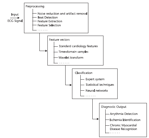Figure 2. ECG Classification process

Figure 3. Block Diagram of system

3. Methodology

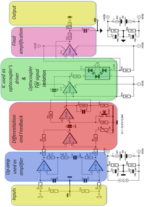
The circuit (Figure 4) can be divided into two blocks: the instrumentation amplifier itself at the input and the optocoupler isolation amplifier at the output. The signal is amplified biquad operational amplifier IC1, type TL084 (or the lower-noise TL074). IC1.A and IC1.B are non-inverting amplifiers, feeding the inputs of differential amplifier IC1.C. This arrangement is known as an ‘instrumentation amplifier’. P1 allows adjustment to obtain best common- mode rejection. Coupling capacitor C3 at the input to the next stage, built around IC1.D, blocks the DC component of the output of the instrumentation amplifier. To minimize the effect on low-frequency signals the time constant of the RC network formed by C3 and R10 is more than three seconds. This means that it will take at least this long for the voltage across the capacitor to stabilize when power is applied: this delay can be avoided by pressing reset button S1. Optocoupler IC3 is driven by IC2. The type TS921 used is a ‘rail to rail’ opamp, which means that it can be driven to either extreme of its supply voltage range. Its output can deliver up to 80 mA, although only approximately 2.2 mA is needed to drive the transmit LED in the optocoupler.

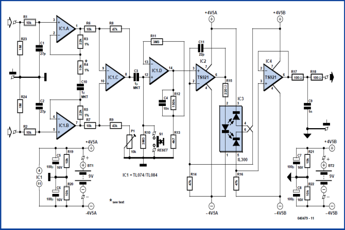Figure 4. Circuit of the instrumentation amplifier

Figure 5. The populated prototype board explained

The current through the transmit LED is controlled using feedback from one of the receiver diodes in the optocoupler fed in to the inverting input of the operational amplifier. The result is that the voltage across R16 (the bias resistor for the second receiver diode) is equal to that across R14 and hence to the voltage at the non-inverting input to IC2. In other words, the voltage at the output of IC1.D appears across R16, but with galvanic isolation. C11 prevents high-frequency oscillation of the driver. The final opamp at the output of the circuit acts as a buffer amplifier. This makes for a low-impedance output, which is also short-circuit proof thanks to the 100 Ω resistors R17 and R18, forming a low-pass filter at the output in combination with C9. The complete galvanic isolation between input and output of the circuit provides for extra safety. The instrumentation amplifier and the output stage should be powered from separate batteries.

3.1. Components and Construction

For resistors R3, R4 and R5 low-noise metal film types were used. C10 provides DC decoupling for the input amplifiers, which prevents weak muscle signals from swamping the signal from the heart. Instead of the tube, disposable self-adhesive ECG electrodes can be used. In order to do so, the capacitor would be replaced by a wire link.

If the TS921 should prove hard to obtain, a type TL071 can be substituted at the cost of reducing the dynamic range of the circuit somewhat. The 43 kΩ resistor (value from the E24 series) can also be replaced by a different value, adjustment of P1 compensating for the difference. IC3 is supplied with its pins bent at a right angle. To fit the circuit board they needed be bent apart (Figure 5): this was necessary in order to guarantee the necessary isolation gap. P1 can be adjusted for best common mode rejection. For best results a connection of the inputs of the instrumentation amplifier and adjustment of P1 to minimize the amplitude at the output of the 50 Hz signal picked up by the circuit was necessary. This measurement can be done using the Matlab program as will be seen later on. The heart signal sensor used for the tests consists of two adapters that can grab naked cables or metallic tips of patches like the ones used for measuring ECG signals onto humans. This is more convenient and makes the device portable with minimum loss of signal and minimum input of undesired noise that could jam the measurements. The same grabbers were used to connect the audio cable that connects the PC to the audio line (or microphone input). Most computers use a 3.5 mm stereo jack.

3.2. New Functions Created for this Research (to read files ECG of ECG hardware)

The first program created to Matlab was about the need to read the signals that are leaded from the output of the construction, to the input of the sound card. This program is consisted from the following lines:

Fs=11025;

Signal=wavrecord(10*Fs,Fs);

These lines are used to read a healthy cardiac signal from the simulator (Rate: 72Bpm) and the output is shown in figure 42. The variable Fs is the waveform rate (11025 KHz) and the 10*Fs are the seconds measured, which are 10 (figure 6).

Figure 6. Output of an SNR

As seen in figure 7, in 10 seconds the simulated heart gave 12 beats. If the measurement is expanded in 60 seconds, the simulator would give 72 heartbeats, which is confirmed from the user manual of the simulator.

Figure 7. The 110250 spots are divided with the waveform rate which was 11.025 KHz and the graphical now is in seconds

This is the basic command that will be used in the program in the graphical interface, so checking and reading of the board is made.

Figure 8. The starting page of the program in which only the drawing output and the box where the insertion of the seconds measured are shown. The “run” button performs the original routine

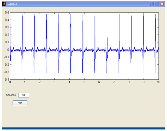Figure 9. Figure 6 as shown in the graphical interface of the program

Next step on the analysis and process of the heart signals is the calculation or the heart rate. In order to do so, a measurement of how many times a higher state in the signal in 10 seconds time is seen, had to be done. Then an escalation of it to 60 seconds is followed. From figure 6 it became obvious that in 10 seconds time the construction measured 12heart beats, thus 72 heart beats per minute (hbpm). For the needs of a fast measure of the heart rate a program that is consisted from the following lines was created:

clc

clear a % to clear a

clear b % to clear b

clear n1 % to clear n1

clear x1 % to clear x1

clear n % to clear n1

clear x % to clear x1

john=0;

x=signal; % x equals our signal

xx=x/max(x); % normalizing amplitude by divide signal with its maximum value

nn=[1:length(xx)]'/11025; % axis x is the length divided by the waveform rate

b=0; % we equal b to zero

a=imextendedmax(xx,1);

for i=2:length(a)-1

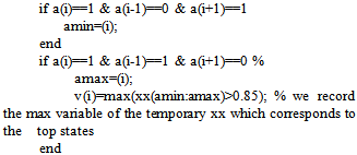end

n1=nn(a);

x1=xx(a);

plot(nn,xx,n1,x1,'r.') % we plot our signal and the top

states it calculated

peaksno=sum(v~=0); % we calculate all of the peaks

Rhythm=(peaksno*60)/length(nn) % we calculate the rate, based on the minutes it recorded.

With the above program calculation of the heart rate and the coding works is made as follows. At first all the variants equals to zero. Then the variable x is stated as the signal and that variable xx is the normalized signal. Next, nn are the numbers of the horizontal axis that define time, in seconds because earlier all of the numbers were divided to 11025 which is the waveform rate (Hz). 1 Hz is 1 circle per second, so 11025Hz are 11025 circles per second, so since the signal has measured 110250 spots, it has counted 10 seconds. Then with command imextendedmax(xx,1); the program equals 1 with all the values that are around the top. In this way, a board (board a) that is consisted by 1 and 0 is created. With commands “for” and “if”, isolation of the entire areas one by one and search the max xx for each one follows. This way “board V” which is consisted by “xx” and “0” is created (where there is not a tag due to non existence of peak, 0 is inserted). Next with command sum(v~=0) all the max values are measured. With Rhythm=(peaksno*60)/length(nn) all the max values from the seconds which the construction measured in 60 in order to define the rate per minutes are escalated. This code was installed to the program in figure 45 along with the capability of the manual calculation of the heart rate. This function was installed due to some cases the heart disorder is so great that the earlier and standard thresholds couldn’t help. Also this capability to manually calculate the heart rhythm in case someone would want to double check the output of the program (figure 10).

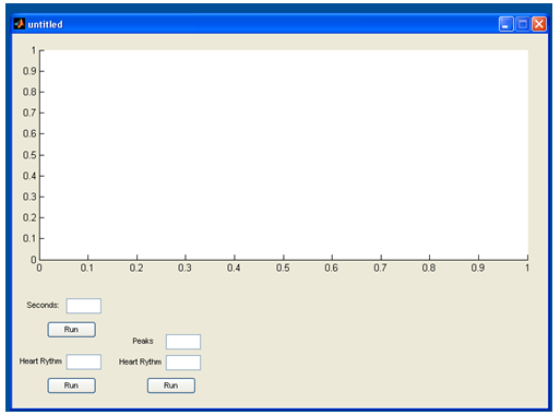Figure 10. The program

4. Conclusions

In this research, signal processing and programs implementation are based in Matlab environment. The processed simulated signal source came from the SIMULAIDS® interactive ECG simulator™ device and the actual heart signals came from actual patients that suffer from various heart disorders, as well as healthy persons that hadn’t recorded any form of heart condition in the past.

For the creation of the database in this research, 5 types of ECG waveform were selected from the ECG simulator device. These are normal sinus rhythm (NSR), ventricular tachycardia (VT poly), ventricular fibrillation (VF), Atrial fibrillation (A FIB) and supra ventricular tachycardia (SVT). An essential part of this research was the development of a portable high resolution ECG device, capable of connecting with, either an ECG simulator device, or recording real human data. This device is able to produce higher resolution than normal ECG devices and high values of Signal to Noise Ratio (SNR).