Mawia Ahmed Hassan1, Yasser Mostafa Kadah2
1Biomedical Engineering Department, Sudan University of Science & Technology, Khartoum, Sudan
2Systems & Biomedical Engineering Department, Cairo University, Giza, Egypt
Correspondence to: Mawia Ahmed Hassan, Biomedical Engineering Department, Sudan University of Science & Technology, Khartoum, Sudan.
| Email: |  |
Copyright © 2012 Scientific & Academic Publishing. All Rights Reserved.
Abstract
Ultrasound imaging is an efficient, noninvasive, method for medical diagnosis. A commonly used approach to image acquisition in ultrasound system is digital beamforming. Digital beamforming, as applied to the medical ultrasound, is defined as phase alignment and summation of signals that are generated from a common source, by received at different times by a multi-elements ultrasound transducer. In this paper first: we tested all signal processing methodologies for digital beamforming which included: the effect of over sampling techniques, single transmit focusing and their limitations, the apodization technique and its effect to reduce the sidelobes, the analytical envelope detection using digital finite impulse response (FIR) filter approximations for the Hilbert transformation and how to compress the dynamic range to achieve the desired dynamic range for display (8 bits). Here the image was reconstructed using physical array elements and virtual array elements for linear and phase array probe. The results shown that virtual array elements were given well results in linear array image reconstruction than physical array elements, because it provides additional number of lines. However, physical array elements shown a good results in linear phase array reconstruction (steering) than virtual array elements, because the active elements number (Aperture) is less than in physical array elements. We checked the quality of the image using quantitative entropy. Second: a modular FPGA-based 16 channel digital ultrasound beamforming with embedded DSP for ultrasound imaging is presented. The system is implemented in Virtex-5 FPGA (Xilinx, Inc.). The system consists of: two 8 channels block, the DSP which composed of the FIR Hilbert filter block to obtain the quadrature components, the fractional delay filter block (in-phase filter) to compensate the delay when we were used a high FIR order, and the envelope detection block to compute the envelope of the in-phase and quadrature components. The Hilbert filter is implemented in the form whereby the zero tap coefficients were not computed and therefore an order L filter used only L/2 multiplications. This reduced the computational time by a half. From the implementation result the total estimated power consumption equals 4732.87 mW and the device utilization was acceptable. It is possible for the system to accept other devices for further processing. Also it is possible to build 16-,32-, and 64-channel beamformer. The hardware architecture of the design provided flexibility for beamforming.
Keywords:
Medical Ultrasound, Digital Beamforming, FIR Hilbert Transform Filter, FPGA, Embedded DSP
Cite this paper: Mawia Ahmed Hassan, Yasser Mostafa Kadah, Digital Signal Processing Methodologies for Conventional Digital Medical Ultrasound Imaging System, American Journal of Biomedical Engineering, Vol. 3 No. 1, 2013, pp. 14-30. doi: 10.5923/j.ajbe.20130301.03.
1. Introduction
Ultrasound is defined as acoustic waves with frequencies above those which can be detected by the ear, from about 20 KHz to several hundred MHz. Ultrasound for medical applications typically uses only the portion of the ultrasound spectrum from 1 MHz to 50 MHz due to the combined needs of good resolution (small wave length) and good penetrating ability (not too high a frequency)[1]. They are generated by converting a radio frequency (RF) electrical signal into mechanical vibration via a piezoelectric transducer sensor[2]. The ultrasound waves propagate into the tissues of the body where apportion is reflected, which used to generate the ultrasound image. Employed ultrasound waves allow obtaining information about the structure and nature of tissues and organs of the body[3]. It is also used to visualize the heart, and measure the blood flows in arteries and veins[4].The commonly use arrays are linear, curved, or phase array. The important distinctions arise from the method of beam steering use with these arrays. For linear and curve linear, the steering is accomplished by selection of a group of elements whose location defines the phase center of the beam. In contrast to linear and curve linear array, phase array transducer required that the beamformer steers the beam with switched set of array elements[5]. These requirements mention important differences in complexity over the linear and curved array. Beamformer has two functions: directivity to the transducer (enhancing its gain) and defines a focal point within the body, from which location of the returning echo is derived.A commonly used approach to image acquisition in ultrasound system is digital beamforming because the analog delay lines impose significant limitations on beamformer performance and more expensive than digitalimplementations. Digital beamforming, as applied to the medical ultrasound, is defined as phase alignment and summation[2] of signals that are generated from a common source, by received at different times by a multi-elements ultrasound transducer[6].The beamforming process needs a high delay resolution to avoid the deteriorating effects of the delay quantization lobes on the image dynamic range and signal to noise ratio (SNR)[7]. If oversampling is used to achieve this timing resolution[8], a huge data volume has to be acquired and process in real time. This is usually avoided by sampling just above the Nyquist rate and interpolating to achieve the required delay resolution[7].Beamforming required Apodization weighted to decreasing the relative excitation near the edges of the radiating surface of the transducer during transmit or receiving, in order to reduce side lobes. Just as a time side lobes in a pulse can appear to be false echoes.After delay and sum the envelope of the signals is detected. The envelope then compressed logarithmically to reduce the dynamic range because; the maximum dynamic range of the human eye is in the order of 30 dB[9]. The actual dynamic range of the received signal depends on the ADC bits, the time gain compensation (TGC) amplifier used in the front end, and the depth of penetration. The signal is compressed to fit the dynamic range used for display (usually 7 or 8 bits). It is typical to use a log compressor to achieve the desired dynamic range for display[10]. With the growing availability of high-end integrated analog front-end circuits, distinction between different digital ultrasound imaging systems is determined almost exclusively by their software component.We develop a compact low-cost digital ultrasound imaging system that has almost all of its processing steps done on the PC side. In this paper first: we tested all signal processing methodologies for digital beamforming which included (Figure 1): the effect of over sampling techniques, single transmit focusing and their limitations, the apodization technique and its effect to reduce the sidelobes, the analytical envelope detection and how to compress the dynamic range to achieve the desired dynamic range for display (8 bits). Here the image was reconstructed using physical array elements and virtual array elements for linear and phase array probe.Second: a modular FPGA-based 16 channel digital ultrasound beamforming with embedded DSP for ultrasound imaging is presented. The system is implemented in Virtex-5 FPGA (Xilinx, Inc.).
2. Methodology
2.1. Over Sampling Technique
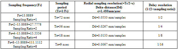
Over sampling is used to achieve high delay resolution. However, this increase the data volume has to acquire. This is usually avoided by sampling just above the Nyquist rate and interpolating to achieve the required delay resolution. Radial sampling resolution is a relationship between the depth and the number of delay values and it equals to the speed of sound over twice the sampling frequency. From the literature[7], wide band transducer required delay resolution in order of 1/16 the signal period.
2.2. Delay Equation
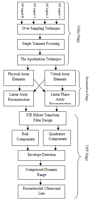 | Figure 1. The technique block diagram |
Figure 2 shows the geometry which is used to determine the channel and depth-dependent delay of a focused transducer array. After a wave-front is transmit into the medium an echo wave propagates back from the focal points (P) to the transducer. The distance from P to the origin is equal to the Euclidian distance between the spatial point (xi,yi) ( is the center for the physical element number i) and the focal point (xf,yf) (is the position of the focal point). The original time, ti, equal the distance from P over the speed of sound. A point is selected on the whole aperture (AP) as a reference (xc,yc) for the imaging process. The propagation time (tc) for this was calculated as the above, but the distance here from P to the reference (xc,yc). The delay to use on each element of the array is the difference between tc and ti. 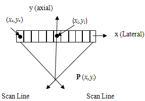 | Figure 2. Geometry of a focused transducer array |
2.3.1. Linear Array Reconstruction
Selected of a group of elements (aperture) whose location is defines the phase center of the beam[1]. Electronic focusing was applied on receive for each aperture. Received at the aperture elements are delayed by focusing delays and summed to form scan line in the image. After that one elements shift is applied to the aperture and the process was repeated till the end of the array elements at the outer side processing all image scan lines (Figure 3 where aperture equal 32 elements). The number of lines equal to the total number of elements minus the number of the aperture elements plus one.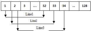 | Figure 3. Linear physical array elements |
2.3.2. Linear phase array reconstruction
In contrast the linear array, phase array transducer required that the beamformer steered the beam with an unswitched set of array elements[1]. In this process, the time shifts follow a linear pattern across of array from one side to another side. In receive mode, the shifted signals are summed together after phase shift and some signal conditioning to produce a single output. This reconstruction technique divides the field of view (FOV) into different point targets (raster points), P(i,j).Each point represented as an image pixel, which is separated laterally and axially by small distances. Each target is considered as a point source that transmits signals to the aperture elements as in figure 4. The beamforming timing is then calculated for each point based on the distance R between the point and the receiving element, and the velocity of ultrasonic beam in the media. Then the samples corresponding to the focal point are synchronized and added to complete the beamforming as the following: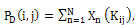 | (1) |
where PD (i,j) is the signal value at the point whose its coordinates are (i,j), and Xn(Kij) is the sample corresponding to the target point in the signal Xn received by the element number n. The sample number Kij which is equivalent to the time delay is calculated using the equation below: | (2) |
Here Rn (i, j) is the distance from the center of the element to the point target, c is the acoustic velocity via the media, and T is the sampling period of the signal data. 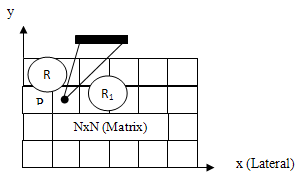 | Figure 4. The raster point technique |
2.4. Virtual Array Elements
2.4.1. Linear Array Reconstruction
In this technique we used central elements and assumed there were virtual elements on the left of the central element. For example, if we want to use aperture equal 128 elements we take element number 1 as center element and selected 64 physical elements on the right (already exist) and 64 virtual elements on the left (not exist), as in figure 5. To compensate the loss in energy, we multiplied by factor (Ma) because this line really taken from 64 elements instead of 128 elements. The Ma factor equal the number of aperture elements divided by the number of the physical elements.Image line was obtained from the summation of physical elements multiplied by Ma factor. There for the Line number one equal the summation of the 64 physical elements × 128/64. Then one elements shift was applied to the virtual and physical aperture and this process is repeated till the factor equal 128/128.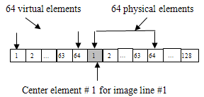 | Figure 5. Linear virtual array elements |
2.4.2. Linear phase array reconstruction
We used the same techniques as in section (2.3.2).
2.5. Apodization
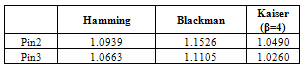
Apodization is amplitude weighting of normal velocity across the aperture[9][11], one of the main reasons for apodization is to lower the side lobes on either side of the main beam[12]. Just as a time side lobes in a pulse can appear to be false echoes[9]. Aperture function needed to have rounded edges that taper toward zero at the ends of the aperture to create low side lobes levels. We used windowing functions (hamming, Blackman, and Kaiser (β=4)) as apodization functions to reduce the side lobes. There is trade-off in selecting these functions: the main lobe of the beam broadens as the side lobes lower[9].
2.6. Envelope Detection and Compressed The Dynamic Range
2.6.1. FIR Hilbert Transform Filter Design
After delay and sum, the analytic envelope of the signal is calculated as the square root of the sum of the squares of the real and quadrature components[13]. The most accurate way of obtaining the quadrature components was to pass the echo signal through a Hilbert transform[14], because it provides 90-degree phase shift at all frequencies[15].The Hilbert transformation filter acts like an ideal filter that removes all the negative frequencies and leaves all positive frequencies untouched. A number of authors suggested the use of digital FIR filter approximations to implement the Hilbert transformation. For linear time invariant (LTI) a FIR filter can be described in this form[16]: | (3) |
Where x is the input signal, y is the output signal, and the constants bi, i= 0,1,2,…,M, are the coefficients. The designed FIR Hilbert filter can be used to generate the Hilbert transformed data of the received echo signal. The impulse response of the Hilbert filter with length N (odd number) is defined as[17]: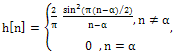 | (4) |
 . We chose the filter length equal 16,20,24,28 and 32-tap with a Hamming window used to reduce the sidelobe effects. According to the normalized root mean square error (RMSE) between the designed FIR Hilbert filter and ideal Hilbert transform filter. The values of the RMSE for the five FIR filters are shown in table 1. We selected 24-tap FIR filter because it provided a good result for the qadrature components compared to ideal
 | Table 1. The Normalized RMSR for FIR Hilbert filters |
| | FIR Hilbert filter order | Normalized RMSE value | | 16 | 0.0109 | | 20 | 0.0096 | | 24 | 0.0092 | | 28 | 0.0091 | | 32 | 0.0090 |
|
|
2.6.2. Compressed the Dynamic Range
The envelope then compressed logarithmically to achieve the desired dynamic range for display (8 bits). It is typical to use a log compressor to achieve the desired dynamic range for display. Log transformation compressed the dynamic range with a large variation in pixels values[18].
2.7. Implementation Steps
 | Figure 6. Architecture implementation of the modular FPGA-Based 16- channel digital ultrasound receive beamformer blocks |
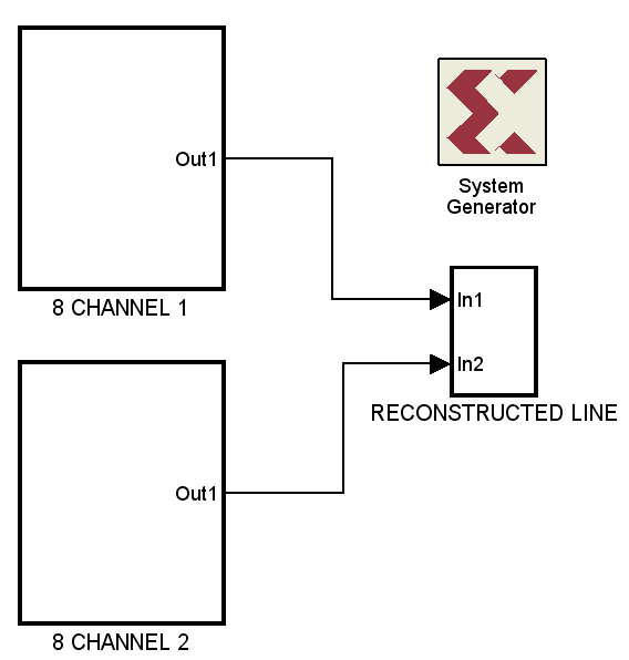
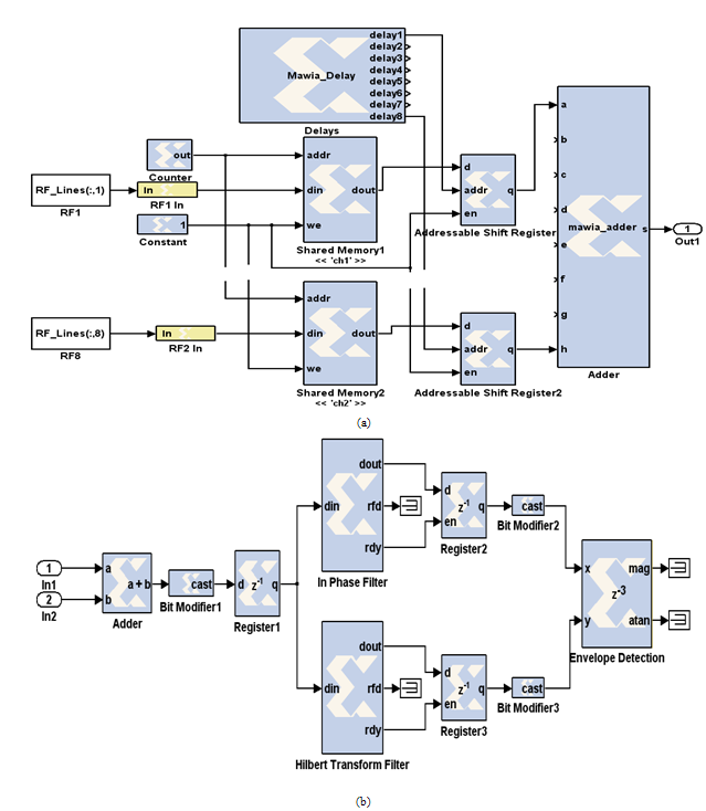 | Figure 7. The inside contents of the implementation blocks. (a) The 8 channel block, (b) the reconstructed line block |
A typical architecture implementation of the modular FPGA-based, 16-channel digital ultrasound receive beamformer with embedded DSP for ultrasound imaging was shown in figure 6. The system consist of: Two 8 channels block and reconstructed line block. The beamfomer is done by using Xilinx system generator (Xilinx, Inc.) and MATLAB simulink (MathWorks, Inc.). The system is implemented in Virtex-5 FPGA. The implementation steps are (Figure 7):1. The RF data saved in MATLAB workspace and used Xilinx block to read the one dimension RF data from workspace.2. The RF data then convert the double precision data type to fixed point numeric precision for hardware efficiency.3. Verified the fixed-point Model by compared the fixed-point results to the floating-point results and determine if the quantization error is acceptable.4. After verified the model, each channel data saved in memory block. The memory word size is determined by the bit width of the channel data. The memory controlled by wire enable port with 1 indicates that the value of the channel data should be written to the memory address pointed to by step-up counter.5. The delay process is based on sampled delay focusing (SDF). The delays calculated using the same method in section 2.2. Then the delays converted to number of samples by divided the delays by the sampling time. SDF consist of addressable shift register (ASR) to delay the sampled signals, and M-Code Xilinx block that contain the calculated delays. The samples are delayed by the value in the address input of the ASR.6. After delaying each RF channel samples, the summation is applied using M-Code block to summate the 8 channel signals.7. The summation of the two 8 channels is connected to adder to reconstructed the final focus line.8. Modify the bit of the signal to 16 bit using the bit modifier block.9. The Register block (data presented at the input will appear at the output after one sample period).10. We used the FIR Hilbert filter (with 24-tap as in section 2.6.1) block for applying the quadrature components.11. The Fractional delay filter (in-phase filter) to compensate the delay when we are being used a high FIR order.12. Then we modified the bit of the signals from step 10 and 11 to 16 bit again using the bit modifier blocks. 13. The Envelope detection block which was computed the envelope of the two signals coming from step 10 and 11.14. In order to obtain performance and logic utilization figures for the suggestion architecture, it was implemented in the hardware description language (VHDL) and synthesized with Virtex-5 FPGA.
3. Results and Discussions
3.1. The Ultrasound data
We used correct data obtained from the Biomedical Ultrasound Laboratory[19], University of Michigan; the phantom data set that was used to generate the results here is under "Acusonl7" and real data (cyst4_a100). The parameters for this data set are as follows: the number of channels was 128 channels, and the A/D sampling rate was 13.8889 MSPS. Linear shape transducer was used to acquire the data with center frequency of 3.5 MHz, and element spacing of 0.22mm. Each ultrasonic A-scan was saved in a record consisted of 2048 RF samples per line each represented in 2 bytes for the phantom data and 4 byte for the real data, and the signal averages was 8. The speed of the ultrasound was 1480 m/sec. The data were acquired for phantom within 6 pins at different positions. The data was used to simulate the N-channel beamformer on receive as discussed in methodologies. The radio frequency (RF) signals, A-scan, were recorded from every possible combinations of transmitter and receiver for all elements in the 128 elements.
3.2. Over Sampling Technique
Table 2 was shown the effect of oversampling to the delay resolution. As can be shown when sampling ratio increased the delay resolution decreased according to the radial sampling resolution. From the table the Delay resolution equal to (1/(2×sampling ratio)).From the table when the sampling ratio (F) equal 8 as an interpolation factor, it gave better delay resolution (1/16) the signal period. However, this increase the data volume has to acquire.
3.3. Physical Elements Array
3.1.1. Linear Array Image Reconstruction
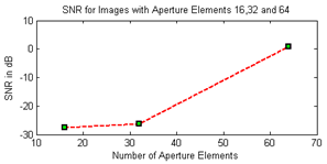
In this situation we reconstructed an image using N-channel beamformer on receive where N=4,8,16,32 and 64. Figure 8 was shown images reconstructed for six pin phantom by linear technique (figure3). In figure 8 (b,c,d and e) the images was reconstructed with focusing using AP equal 4,8,16,32and 64. In figure 8 (a) image was reconstructed without focusing and AP=4 elements. When the AP size increased the lateral resolution was improved. However, the FOV was reduced when the aperture size increased. Figure 9 shown the signal to noise ratio (SNR) when aperture equal 4,8,16,32,and 64. As can be shown when the size of AP increased that improved the SNR. Also figure 10 described the effect of oversampling technique. Table 2. The effect of the oversampling to the delay resolution
 |
| |
|
Here we used image with AP equal to 64 with F equal to 1,2,4,and 8 then we calculated the SNR for each images. As can be shown The SNR was improved when the F increase.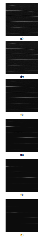 | Figure 8. Physical Linear array image reconstruction, (a) Using AP=4 without focusing, (b) Using AP=4 with focusing, (c) Using AP=8with focusing, (d) Using AP=16 with focusing, (e) Using AP=32 with focusing, (f) Using AP=64 with focusing |
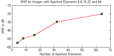 | Figure 9. SNR for AP equal 4,8,16,32,and 64 using physical linear array |
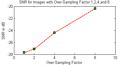 | Figure 10. The effect of oversampling technique to the SNR. Here we used image with AP equal to 64 with F equal to 1,2,4,and 8 |
3.3.2. Linear Phase Array Reconstruction
Due to the small FOV of the linear reconstruction and its limited lateral resolution, we used linear phase reconstruction to reconstructed image of six pins phantom from the data set. Figure 11 shown images reconstructed using raster point technique. Element number 128 was the transmitter and received with all 128 elements. In figure 11 (a and b) image was reconstructed using F equal 4 and 8. As we saw when F was increased it improved the image quality because from table 1 radial resolution equals 0.0067 for (F=8) compared to 0.0133 for (F=4). Figure12 shown image reconstructed by the same technique using all elements for transmitted and received. The six pin of the phantom are clearly described with a moderate lateral resolution.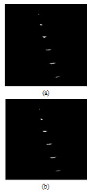 | Figure 11. Physical Linear phase array image reconstruction, element number 128 for transmitted and received with all 128 elements, (a) Using F=4, (b) Using F=8 |
 | Figure12. Physical Linear phase array image reconstruction, transmitted and received with all 128 elements (a) Using F=4, (b) Using F=8 |
3.4. Virtual Array elements
3.4.1. Linear Array Image Reconstruction
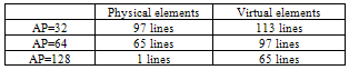
Table 3 shown a comparison between linear array reconstruction with physical and virtual elements, as can be seen virtual elements provide additional scan lines leaded to improved the FOV and lateral resolution than using physical array elements. Also virtual array elements provided a possibility of using AP equal 128 elements with 65 lines and that could not be acceptable in physical array elements, because we had only one line. Table 3. Number of lines in linear array image reconstruction with physical and virtual elements
 |
| |
|
Figure 13 showed 32, 64, and 128 elements channel beamformers. Figure 13 (a and b) shown 32 and 64 channel respectively, as can be shown, when increased the AP the lateral resolution was improved and also FOV been better than physical array elements in figure 8 (e and f). In figure 13 (c) the AP equal 128 which it's unacceptable in physical array elements.
3.4.2. Linear Phase Array Reconstruction
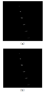
Figure 14 (a, b, and c) shown images reconstructed using raster point technique for virtual elements when AP equal 32, 64, and 128 elements respectively. As we saw virtual elements array in steering reduced the FOV but the lateral resolution was good compared to the physical array elements which gave a good FOV and lateral resolution. Figure 15 shown the SNR when AP equal 16,32,and 64. As can be shown when the size of AP increased the SNR was improved.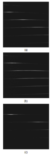 | Figure 13. Virtual linear array image reconstruction, (a) Using AP=32, (b) Using AP=64, (c) using AP=128 |
 | Figure 14. Virtual Linear phase array image reconstruction, (a) Using AP=32, (b) Using AP=64,(c) AP=128 |
 | Figure 15. SNR for AP equal 16,32,and 64 using raster point technique for virtual elements |
3.5. Effect of Apodization
Table 4 shown the effect of Hamming, Blackman, and Kaiser (β=4) apodization windows compared to rectangular window. Because the aperture is rectangular unfortunately, the far field beam pattern is a sinc function with near in-side lobes only -13 dB down from the maximum on axis value.From table 4 there is trade-off in selecting these functions: the main lobe of the beam broadens as the side lobes lower. Also the table described the SNR between these windows. As can be shown the Blackman apodization function was given a better SNR, better reduction in the sidelope and good main lobe width compared to the other windows.| Table 4. Hamming, Blackman, and Kaiser (β=4) apodization functions compared to rectangular window (without Apodization) |
| | Type of Window | Peak Side Lope Amplitude(Relative) | Approximate Width of Main Lobe | SNR (Relative) | | Rectangular | -13.3 | 0.0137 | 32.6680 | | Hamming | -42.6 | 0.0195 | 37.6472 | | Blackman | -58.1 | 0.0252 | 38.4245 | | Kaiser (β=4) | -30.0 | 0.01758 | 37.0413 |
|
|
Figure 16 was shown a comparison between images reconstructed without apodization using physical array elements (transmitted and received by all elements) to images reconstructed with apodization. As can be shown in figure 16 (b, c, and d) there is trade-off in selecting these functions: the main lobe of the beam broadens as the side lobes lower compared to figure 16(a) for rectangular aperture.
3.6. Envelope Detection and Compressed Dynamic Range
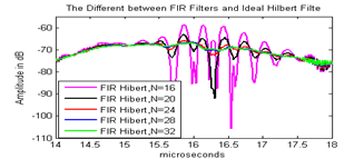
The frequency response of apply 16-, 20-, 24-, 28-, and 32-tap FIR Hilbert filter shown in Figure 17. Figure 18 had shown the different between the FIR Hilbert filters and the ideal Hilbert filter. The normalized root mean square error (RMSE) between the FIR hilbert filter and ideal Hilbert transform filter for the five FIR filters are shown in table 1. From the result 24-tap provided a good result because it gave the medium RMSE (0.0092) between the five selected FIR filters that it gave a good result because the different between it and the ideal Hilbert filter look like random signal.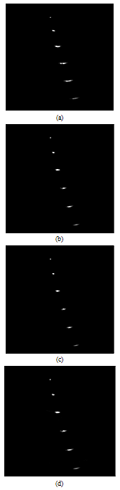 | Figure 16. Comparison between images reconstructed with and without apodization. (a) Image without apodization, (b) Image apodized with Hamming,(c) Image apodized with Blackman,(d) image apodized with kaiser (β=4) |
Fig.19 was shown comparisons between envelope images used physical and virtual linear array elements. In figure 19(a and b) image reconstructed using aperture equal 32 and 64 with physical array and fig.19(c, d, and e) shown images reconstructed using aperture equal 32, 64, and 128 respectively with virtual elements. As can be shown virtual elements array provide best FOV and lateral resolution than physical array elements. 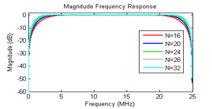 | Figure 17. The frequency response of apply 16-, 20-, 24-, 28-, and 32-tap FIR Hilbert filter |
 | Figure 18. The different between the FIR Hilbert filters and the ideal Hilbert filte |
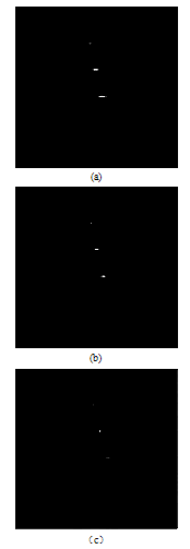
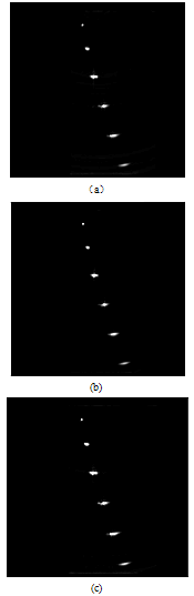
In figure 20 we shown the envelope of images used raster point technique (There were 128 elements for transmits and receives), apodized by Hamming, Blackman, and Kaiser (β=4) respectively. As can be viewed the results were better than figure 16 (b,c, and d), because the envelope provided more signal strength as can be shown in figure 21.The same was also said for figure 19 (a and b) compared to figure 8 (e and f) and figure 19 (c,d, and e) compared to figure 13 (a,b,and c).Figure 22 (a,b, and c) shown the images in figure 20 (a, b, and c), which compressed the dynamic range using logarithmic compression to achieve the desired dynamic range for display (8 bits).Figure 23 and figure 24 had shown an image line with and without compress the dynamic range. As can be shown the maximum dynamic range without compress equal to 105dB and 13dB after compress the dynamic range.Figure 25 (a) shown pin three in the compressed image as a sub-image without apodization. Figure 25 (b, c, and d) shown the same pin apodized by Hamming, Blackman, and Kaiser (β=4) respectively. Figure 25 (e, f, and g) was a lateral profiles shown the effect of apodization to the side lobes and main lobe as function in the frequency domain. As can be shown there is trade-off in selecting these functions: the main lobe of the beam broadens as the side lobes lower.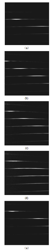 | Figure 19. Comparisons between envelope images used physical and virtual linear array elements (a) Image with physical array elements using AP=32, (b) Image with physical array elements using AP=64, (c) Image with virtual elements using AP=32, (d) Image with virtual elements using AP=64, (e) Image with virtual elements using AP=128 |
Fig.26 shown images reconstructed using raster point technique for real data (Cyst). The over sampling factor (F) equal 8, apply the envelope detection to over sampling data and compressed the dynamic range used Log compression.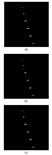 | Figure 20. The envelope images used raster point technique (There were 128 elements for transmits and receives) (a) Envelope image apodized with Hamming , (b) Envelope image apodized with Blackman , (c) Envelope image apodized with Kaiser (β=4) |
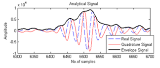 | Figure 21. The analytical envelope |
 | Figure 22. The compressed envelope images used log compression (transmitted and received with all elements) (a) Compressed envelope image apodized with Hamming , (b) Compressed envelope imageapodized with Blackman , (c) Compressed envelope image apodized with Kaiser (β=4) |
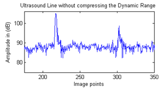 | Figure 23. The dynamic range without compression |
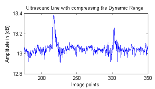 | Figure 24. The dynamic range with compression |
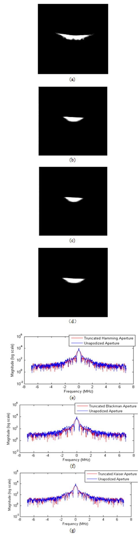 | Figure 25. Pin three in the phantom as a sub-image. (a) Without apodization,(b) Apodized with Hamming , (c) Apodized with with Blackman , (d) Apodized with Kaiser (β=4), (e) Frequency spectrum of fig.24 (b), (f) Frequency spectrum of fig.24 (c), (e) Frequency spectrum of fig.24 (d) |
 | Figure 26. Image reconstructed using raster point technique for real data (Cyst) |
3.8. Image Quality
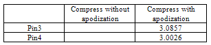
We selected pin number two and pin number three as sub-images (64X64) and (100X100) respectively, to show the quality of the images using an entropy function. Table 5 was shown a comparison of images quality (entropy) without apodization (figure 16(a)) and image with apodization (figure 16 (b)), Apodization was done using Hamming window. Table 6 was shown entropy of images without apodization (figure 16 (a)) and image apodized with Blachman window (figure 16 (c)). Table 7 was shown an entropy of image without apodization (figure 16(a)) and image with apodization (figure 16 (d)). Apodization was done using Kaiser (β=4) window.Table 5. Entropy of sub-images with apodization (Hamming) and without apodization
 |
| |
|
Table 6. Entropy of sub-images with apodization (Blackman) and without apodization
 |
| |
|
Table 7. Entropy of sub-images with apodization (Kaiser(β=4)) and without apodization
 |
| |
|
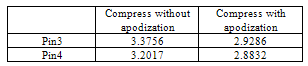
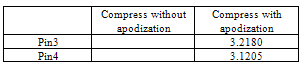
From the tables entropy of image is minimized when the image was uniform. Image with apodization was given entropy value less than image without apodization, indicated for suppressed side lopes. Table 8 was shown an entropy ratio between compressed sub-image without apodization and with apodization. As can be seen Blackman given better results than Hamming and Kaiser in compressed image with apodization.Table 8. An entropy ratio between compressed sub-image without apodization and with apodization
 |
| |
|
3.9. Implementation
3.9.1. Verify the Fixed-point Model
Figure 27 shown double precision RF data type read from MATLAB work space compared to fixed point RF data type for hardware efficiency. We verified the fixed-point Model by subtract the fixed-point RF signal from the floating-point RF signal and the result equal zero. This means zero quantization error.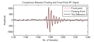 | Figure 27. Comparison between floating and fixed point RF signal |
3.9.2. Delays
Figure 28 (a) and Figure 28 (b) illustrated 100 samples from channel 8 and channel 9 data respectively before and after synchronization. As can be shown in Figure 28(a) the time of arrival is different for the two channel compared to Figure 28(b) with the same arrival times.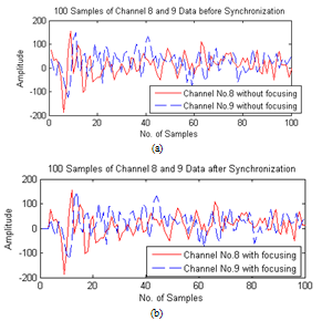 | Figure 28. Alignment for RF signals.(a) 100 samples of channel 8 and 9 before synchronization,(b) 100 samples of channel 8 and 9 after synchronization |
3.9.3. The Reconstructed Line
Figure 29 shown the comparison between implemented the first line (after the pipe line adder in Figure 7 (b)) in image reconstruction and the simulated one. As we mentioned in the methodologies the normalized RMSE between the designed filter and ideal Hilbert transform filter of 24 order FIR Hilbert filter is the medium one (0.0092) , so we use this filter for the simulation and implementation of the ultrasound data. Apply this designed Hilbert filter to the received echo line after delay and sum shown in Figure 30(a) compared to the ideal Hilbert filter in Figure 30 (b). Figure 30 (c) had shown the different between the reconstructed and ideal Hilbert. Figure 30 (d) described the frequency spectrum for ultrasound data. As can be shown the negative frequency was eliminated compared to the ideal Hilbert filter frequency spectrum (Figure 30(e)). Figure 31 had shown the implemented of the linear phase array image reconstruction to reconstruct image of six pins phantom from the data set, and the point spread function (PSF) of the first pin as indicated by white arrow in Figure 31 (b) and Figure 31 (d). Figure 31 (a) described the image reconstruction after delay and sum and Figure 31(c) shown the image reconstructed after applying FIR Hilbert filter and envelope detection. As can be shown Figure 31(c) provided best FOV and lateral resolution than Figure 31 (a), because the envelope provided more signal strength. The PSF presented a quantitative measure of the beamforming quality.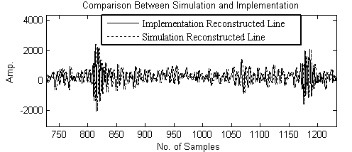 | Figure 29. Comparison between implemented the first line (after the pipe line adder in Fig.6(b)) in image reconstruction and the simulated one |
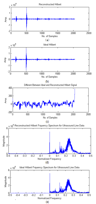 | Figure 30. Hilbert filter apply to ultrasound line data. (a) Reconstructed FIR Hilbert, (b) Ideal Hilbert, (c) the different between the reconstructed and ideal Hilbert, , (d) frequency spectrum of reconstructed FIR Hilbert,(e) The ideal Hilbert filter frequency spectrum |
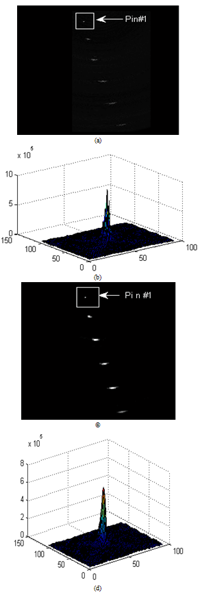 | Figure 31. Image reconstruction and the PSF of the first pin. (a) Image after delay and sum, (b) PSF of the first pin in (a), (c) Image after applying FIR Hilbert filter and envelope detection, (d) PSF of the first pin in (c) |
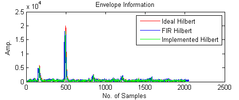 | Figure 32. Comparison between envelope take after apply simulated ideal Hilbert filter ,the 24-tap simulated FIR Hilbert filter and implemented envelope take after apply the 24-tap implemented FIR Hilbert for all the ultrasound line data |
Table 9. 2x system clock (discrete pulse generator)
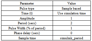 |
| |
|
Table 10. 2x system clock (discrete pulse generator)
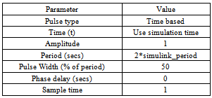 |
| |
|
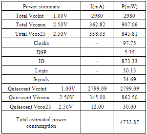
Table 11. Summary of the power consumption in the whole implementation
 |
| |
|
3.9.4. Envelope Detection
Figure 32 described the comparison between envelope take after apply simulated ideal Hilbert filter ,the 24-tap simulated FIR Hilbert filter and implemented envelope take after apply the 24-tap implemented FIR Hilbert for all the ultrasound line data. The result was good if it compared to the simulation results.
3.9.5. Timing and Clock System
Table 9 and 10 were shown the 2x system clock (Discrete Pulse Generator) and continuous source (Discrete Pulse Generator).
3.9.6. Power Consumption
Table 11 was shown the summary of the power consumption in the whole implementation. The total estimated power consumption equal 4732.87 mW.
3.9.7. Device Utilization
Table 12 was shown the device utilization summary for the whole implementation, the used devices, available in the port, and the utilization in percentage using Virtex-5 FPGA.
4. Discussions
From the results when increasing the oversampling ratio this improved the delay resolution but increased the hardware volume in the implementation. A further problem in conventional imaging is the single transmit focus, so that the imaging is only optimally focused at one depth. This can be overcome by making compound imaging using a number of transmit foci, but the frame rate is then correspondingly decreased. One alternative is to use synthetic aperture imaging. The main reason for apodization is to lower the side lobes on either side of the main beam. Just as a time side lobes in a pulse can appear to be false echoes but there is trade-off in selecting these functions: the main lobe of the beam broadens as the side lobes lower. Here the image was reconstructed using physical array elements and virtual array elements for linear and phase array probe. The results shown that virtual array elements were given well results in linear array image reconstruction than physical array elements, because it provides additional number of lines. However, physical array elements shown a good results in linear phase array reconstruction (steering) than virtual array elements, because the active elements number (Aperture) is less than in physical array elements. From the implementation results we shown that the fixed-point Model is the same as the floating point mode and this is an important for hardware efficiency. Future, the delays applied as SDF gave a synchronous in the time of arrival. Furthermore, The Hilbert filter is implemented in the form whereby the zero tap coefficients were not computed and therefore an order L filter used only L/2 multiplications. This reduced the computational time by a half. The total estimated power consumption equal to 4732.87 mW and the device utilization was acceptable.Table 12. Device utilization summary
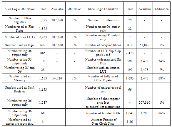 |
| |
|
5. Conclusions
In this work we applied all signal processing methodologies for traditional digital ultrasound beamforming. We used two types to reconstruct the ultrasound images; virtual array elements and physical array elements for linear and phase array probe, then we studied the effect of each one. A modular FPGA-based 16 channel digital ultrasound beamforming with embedded DSP for ultrasound imaging is presented. The system is implemented in Virtex-5 FPGA (Xilinx, Inc.). The computational time was reduced by a half because we implemented the Hilbert filter in the form whereby the zero tap coefficients were not computed and therefore an order L filter used only L/2 multiplications. From the implementation result the total estimated power consumption and the device utilization were acceptable. It is possible for the system to accept other devices for further processing. Also it is possible to build 16-,32-, and 64-channel beamformer. The hardware architecture of the design provided flexibility for beamforming.
References
| [1] | D. A .Christensen, Ultrasonic Bioinstrumentation, Jonh Wiley & Sons, New York, (1988). |
| [2] | J. A Zagzebski , Essentials of ultrasound physics, St Louis, Mo: Mosby, (1996). |
| [3] | W. N.McDicken, Diagnostic Ultrasonics: Principals and Use of Instruments, JohnWiley & Sons, (1976). |
| [4] | S. Hughes, Medical ultrasound imaging, Electronic Journals of Physics Education. 36 ,468–475(2001). |
| [5] | K. E. Thomenius, “Evaluation of Ultrasound Beamformers,” in Proc. IEEE Ultrason. Symp., pp.1615-1621, 1996. |
| [6] | R. Reeder, C. Petersen, The AD9271-A Revolutionary Solution for Portable Ultrasound, Analog Dialogue,Analog Devices. (2007). |
| [7] | C. Fritsch, M. Parrilla, T. Sanchez, O. Martinez, “Beamforming with a reduced sampling rate,” Ultrasonics, vol. 40, pp. 599–604, 2002. |
| [8] | B. D. Steinberg, “Digital beamforming in ultrasound,” IEEE Transactions on Ultrasonics, Ferroelectrics and Frequency Control, vol. 39, pp. 716–721, 1992. |
| [9] | Szabo, T. L., Diagnostic Ultrasound Imaging: Inside Out, Elsevier Academic Press: Hartford, Connecticut, 2004. |
| [10] | M. Ali, D. Magee and U. Dasgupta, “Signal Processing Overview of Ultrasound Systems for Medical Imaging,” SPRAB12, Texas Instruments, Texas, November 2008. |
| [11] | J. A. Jensen, “Ultrasound imaging and its Modeling”, Department of Information Technology, Technical University of Denmark, Denmark, 2000. |
| [12] | J. Synnevag, S. Holm and A. Austeng, “A low Complexity Delta-Dependent Beamformer,” in Proc. IEEE Ultrason. Symp., pp.1084-1087,. 2008. |
| [13] | J. O. Smith, Mathematics of the Discrete Fourier Transform (DFT), Center for Computer Research in Music and Acoustics (CCRMA), Department of Music, Stanford University, Stanford, California, 2002. |
| [14] | A. V. Oppenheim and R. W. Schafer, Discrete-Time Signal Processing. NJ: Prentice-Hall, Englewood Cliffs, 1989. |
| [15] | B.G. Tomov and J.A. Jensen, “Compact FPGA-Based Beamformer Using Oversampled 1-bit A/D Converters,” IEEE Transactions on Ultrasonics, Ferroelectrics and Frequency Control, vol. 52, no. 5, pp. 870-880, May 2005. |
| [16] | J. O. Smith, Mathematics of the Discrete Fourier Transform (DFT), Center for Computer Research in Music and Acoustics (CCRMA), Department of Music, Stanford University, Stanford, California, (2002). |
| [17] | S. Sukittanon, S. G. Dame, FIR Filtering in PSoC™ with Application to Fast Hilbert Transform, Cypress Semiconductor Corp., Cypress Perform. (2005). |
| [18] | R. C. Gonzalez, R. E. Woods, Digital Image Processing, Pearson Prentice Hall, Upper Saddle River, New Jersey, 2008. |
| [19] | M. O’Donnell and S.W. Flax, “Phase-aberration correction using signals from point reflectors and diffuse scatterers: measurements,” IEEE Trans. Ultrason., Ferroelect., and Freq. Contr. 35, no. 6, pp. 768-774, 1988. |
 Abstract
 Reference
 Full-Text PDF
 Full-text HTML