1. Introduction

According to World Health Organization (WHO), suicide is an act of self-killing[1]. However, it could be prevented by judging the ‘intent’ at an appropriate time[2].Yearly about 1 million people commit suicide[3]. It is one of the first 20 leading cause of death[3]. The rate of suicide is quite high, estimated one in every 40 seconds[4]. It has been noted through series of studies that in the last 45 years suicide rates have been increased by 60% across the world[4]. It is the third leading cause of death among people aged between 15 and 44 years and second leading cause of death among those who are 10-24 years of age[4]. Attempting suicide is 20 times higher than actually committing it[4]. Cumulatively suicide caters about 1.8% of total global burden of disease in 1998 and the predicted value would be 2.4% by the end of 2020[4]. Therefore, suicide has a well recognized significance from the public health perspective.

Mental illnesses, such as depression, schizophrenia, personality disorders, alcoholism are some of the most dominating ‘intent’ factors of suicide[3]. Some other important causes are unemployment[5], poverty[6], chronic illnesses[7][8], familial tendencies[9], substance abuse[10] and so forth. Usually the subjects are treated for these disorders. In this context it is important to note that there is no concrete evidence to prove that medications and psychological treatments given to these populations actually reduces the vulnerability of suicide or not. While surveying the literature, it may be noted that most of the randomized control trials related to suicide prevention have failed to yield complete information about the suicidal trends[11]. It is because of the fact that these studies are targeted to a specific population composed of possibly a homogeneous group of subjects[12]. Researchers also believe that randomized control trial of suicide-prone individuals to a treatment condition might be unethical as it could be too much risky[12]. Moreover, there are no available valid measures of suicidal behaviour or ideation. Hence, the research scopes in suicide study are mostly confined to ‘interventions’ using standardized assessment instruments, which are able to measure the variations in the course of suicidality. Based on the nature of the course, treatments might be better planned. The most important of all is that the early recognition of the ‘intent’ which is reflected through emotional and physical sign-symptoms. However, early recognition of ‘intent’ is a difficult task. This is because of the facts that the onset of new symptoms or changes in the earlier symptoms often remains unnoticed and immeasurable. Therefore, routine screening of vulnerable population is the only way to mine such risk and its level/severity.

There are several assessment tools for the screening of suicide[13]. Screening is conducted by interviewing the subjects. The correctness of the interpretation depends on the quality and quantity of the information and the experience level of the interviewers. It is important to note that the experience and the perceptual abilities of the interviewer are completely individualized phenomena and because of it some degrees of variations might be seen in the final ‘intent’ scoring. Another issue is that, such interpretations could be biased as biasness is another considerable human factor that may influence the scoring process. Due to these prevailing issues, suicide is often under or over treated. As a result, the incidences are increasing in the population despite of commendable progress in mental healthcare.

Given this scenario, the objective of this study is to mathematically model and automate the suicidal ‘intent’ classification task using artificial neural network. Beck’s Suicide Intent Scale (BSIS)[14] has been used to construct and validate the networks. It has three major constructs and under these constructs there are total 20 indicators. Each indicator has three preconditions, which are individually assessed during the interview and scored. The first, second and third preconditions are scored as ‘0’, ‘1’, and ‘2’, respectively. Final scoring is the sum of all scores. BSIS structure has been discussed in detail in section 2. The paper also aims to investigate the influence of the ‘number’ (i.e., quantity) and the ‘significance’ (i.e., the quality) of the indicators on suicidal ‘intent’ classification using neural networks. Summarily, the paper attempts to fit BSIS and its interpretation into neural networks. It is discussed in detail under section 3.

Rest of the paper is organized as follows. The structure and interpretation of BSIS has been elaborated in section 2. Real-life data collection, techniques used for the analysis of the data, and the development of Multilayer Feed forward Neural Networks (MLFFNN) to automate the suicide ‘intent’ classification task are described in section 3. Section 4 shows the experiments, related results and its interpretations. Finally, the paper concludes and shows some future directions in section 5.

2. Beck’s Suicide Intent Scale (BSIS)[14]

Aron T. Beck et al., (1974) developed a scale based on the seriousness of suicidal ‘intent’ or will[15][16]. It is administered to the suicide attempters through personal interviews to assess the verbal and nonverbal behaviours prior to and during the most recent suicide attempts. The scale is structured into three major constructs, such as ‘Objective Circumstances Related to Suicide Attempt’ (which covers the objective circumstances reflecting the preparation), ‘Self report’ (which measures the lethality of the acts), and ‘Other aspects’ (which reflects the passive influences, e.g., drugs, alcohols etc., subjects’ reactions following an attempt and so forth). Each construct is composed of several indicators or item or factors, shown in Table 1. In this table, column headings are the major constructs. Under each construct there are the indicators (italicized). The load of each indicator is then assessed with three preconditions (which are star marked) and the corresponding score or ratings of each precondition are assigned within parenthesis to quantify the ‘intent’ loads [17].

Under the first construct, there are eight indicators such as Isolation (I), Timing (T), Precautions againstdiscovery/intervention (PADI), Acting to get help during/after attempt (AH), Final acts in anticipation of death (FAD), Active preparation for attempt (APA), Suicide Note (SN), and Overt communication of intent before the attempt (OCI). On the other hand, Alleged purpose of attempt (AP), Expectations of fatality (EF), Conception of method's lethality (CML), Seriousness of attempt (SA), Attitude toward living or dying (ATLD), Conception of medical rescuability (CMR), and Degree of premeditation (DP) fall under the second construct (see table 1). Actual scoring is performed with these fifteen indicators under the first two constructs due to sufficient inter-rater reliability with Cronbach’s alpha between 0.81 to 0.91[18]. However, there is a third construct, called ‘Other aspects’ possesses five indicators, such as Reaction to attempt (RA), Visualization of death (VD), Number of previous attempts (NPA), Relationship between alcohol intake and attempt (RAA), and Relationship between drug intake and attempt (RDA), which are usually excluded from the scoring as all these are passive or indirect features of the ‘intent’.

Final scoring: Final scoring is done by summing up the scores of the preconditions under the indicators. For example, all the first preconditions are scored as ‘0’, second conditions as ‘1’, and the third conditions as ‘2’ (see Table 1). Scoring is done during interviewing the subjects. Sum scores from 15-19 denote ‘Low Intent’, while 20-28 refer to ‘Medium Intent’, and score more than 29 points towards ‘High Intent’ of committing suicide. The intent usually increases with the numbers of attempts. In this dataset, it has been estimated that 60.5% patients have ‘Low’ intent (i.e. there is one attempted suicide), 37.5% have ‘Medium’ intent (i.e. having history of two suicidal attempts), and 2% possesses ‘High’ intent (i.e. having more than 2 suicidal attempts). Between any two consecutive attempts, the average time span is 6.7 months for this dataset.

3. Materials and Methods

This section discusses various processes adopted in this work. These are as follows.

1) Data collection

2) Data analysis, and

3) Development of Multilayer Feed forward Neural Networks (MLFFNN) to automate the ‘intent’ classification task.

3.1. Data Collection

Capturing warning signs and symptoms (i.e. the data) of suicide ‘intent’ is the most important task to understand the possibility of suicide attempts[19][20]. In this study, the information has been captured from patients’ data sheets (n = 200) and structured using BSIS (described in section 2.2 in table 1). The subjects have been interviewed by experienced medical doctors (mean level of experience is about 6.8 years).

Table 1. Structure of Beck’s Suicide Intent Scale (BSIS)[14] ‘Objective circumstances related to suicide attempt’ ‘Self report’ ‘Other aspects’ 1. Isolation (I):*Somebody present (0)*Somebody nearby, or in visual or vocal contact (1)*No one nearby or in visual or vocal contact (2) 1. Alleged purpose of attempt (AP):*To manipulate environment, get attention, get revenge (0)*Components of above and below (1)*To escape, surcease, solve problems (2) 1. Reaction to attempt (RA):*Sorry it was made; feels foolish; ashamed (0)*Accepts both attempt and failure (1)*Regrets failure of attempt (2) 2. Timing (T):*Intervention is probable (0)*Intervention is not likely (1)*Intervention is highly unlikely (2) 2. Expectations of fatality (EF):*Thought that death was unlikely (0)*Thought that death was possible but not probable (1)*Thought that death was probable or certain (2) 2. Visualization of death (VD):*Life after death, reunion with descendants (0)*Never-ending sleep, darkness, end of things (1)*No conceptions of or thoughts about death (2) 3. Precautions against discovery/intervention (PADI):*No precautions (0)*Passive precautions (as avoiding other but doing nothing to prevent their intervention; alone in room with unlocked door) (1)*Active precautions (as locked door) (2) 3. Conception of method's lethality (CML):*Did less to self than he or she thought would be lethal (0)*Wasn't sure if what s/he did would be lethal (1)*Equalled or exceeded what s/he thought would be lethal (2) 3. Number of previous attempts (NPA):*None (0)*One or two (1)*Three or more (2) 4. Acting to get help during/after attempt (AH):*Notified potential helper regarding attempt (0)*Contacted but did not specifically notify potential helper regarding attempt (1)*Did not contact or notify potential helper (2) 4. Seriousness of attempt (SA):*Did no seriously attempt to end life (0)*Uncertain about seriousness to end life (1)*Seriously attempted to end life (2) 4. Relationship between alcohol intake and attempt (RAA):*Some alcohol intake prior to but not related to attempt; reportedly not enough to impair judgment, reality testing (0)*Enough alcohol intake to impair judgment; reality testing and diminish responsibility (1)*Intentional intake of alcohol in order to facilitate implementation of attempt (2) 5. Final acts in anticipation of death (will, gifts, insurance) (FAD):*None (0)*Thought about or made some arrangements (1)*Made definite plans or completed arrangements (2) 5. Attitude toward living or dying (ATLD):*Did not want to die (0)*Components of above and below (1)*Wanted to die (3) 5. Relationship between drug intake and attempt (RDA):*Some drug intake prior to but not related to attempt; reportedly not enough to impair judgment, reality testing (0)*Enough drug intake to impair judgment; reality testing and diminish responsibility (1)*Intentional intake of drug in order to facilitate implementation of attempt (2) 6. Active preparation for attempt (APA);*None (0)*Minimal to moderate (1)*Extensive (2) 6. Conception of medical rescuability (CMR):*Thought that death would be unlikely if he received medical attention (0)*Was uncertain whether death could be averted by medical attention (1)*Was certain of death even if he received medical attention (2) 7. Suicide Note (SN):*Absence of note (0)*Note written, but torn up; note thought about (1)*Presence of note (2) 7. Degree of premeditation (DP):*None (0)*Impulsive suicide contemplated for three hours of less prior to attempt (1)*Suicide contemplated for more than three hours prior to attempt (2) 8. Overt communication of intent before the attempt (OCI):*None (0)*Equivocal communication (1)*Unequivocal communication (2)

Table 2. Overview of the data collection Sample size 200 Age group 18-50 yrs. Number of males 100 Number of females 100 Mental illness Yes (Schizophrenia = 50, Major depression = 41, Impulsive personality disorder = 43, Depression with psychotic disorders = 26, Obsessive compulsive disorder = 20, and Substance abuse disorder = 20) Number of attempts Max: 4; Min: 1; Mean: 1.65 Average time span between two successive attempts Males: 7 monthsFemales: 4 months Ethical measures Anonymous data and source Observation Retrospective, i.e. assessing the verbal and nonverbal behavior of the latest attempts. Suicidal intent class Low (when one attempt), Medium (two attempts), and High (more than two attempts) Time taken to complete the data collection process 1 yr. (mean 11.2 minutes per interview) Number of interviewers 2 (mean experience level 6.8 yrs.) Preprocessing Done with redundancy, error and missing value checks Reliability of the data Cronbach’s alpha measure.

The reason for choosing BSIS is that it is reliable, easy executable, having high inter-rater reliability, and possesses higher predictive value.

In this work, suicide ‘intent’ levels are assigned as ‘low’, ‘medium’, and ‘high’ according to the number of suicidal attempts. Low intent refers to one attempt, while medium and high intents denote two and more than two attempts, respectively with an average time span of slightly higher than 6 months between any two consecutive attempts.

Appropriate ethical measures have been taken to collect and store the data preserving the privacy of the patients and the sources. Two senior psychologists have helped to organize the data. Time taken to collect the data is approximately 1 year.

Two hundred males and females each between 18 to 50 years of age has been considered in this study as this age group poses to be the most predominant threat. The collected data has finally been checked for redundancies, missing values and errors. Table 2 displays the overview of data collection.

3.2. Data Analysis Using Minitab-14

Data analysis is broadly composed of data preprocessing and processing techniques. It actually helps model abstraction from the dataset. By data analysis valid and interesting patterns within the data could be noted within the abstracted model. Such patterns might be helpful in designing the knowledge-enabled systems for the decision making. In this study, the collected data has been carefully checked for errors, redundancies, and missing values. Cronbach’s alpha[21] has been measured to check the reliability of the data. The threshold of alpha is 0.7[22]. After the initial check, the following tasks are performed to analyze it using Minitab-14[23].

● Examining data distribution by measuring means, standard deviations, and skewness (see table 2 in section 3).

● Viewing the distributions of intent scores among males and females with a scatter plot.

● Analysis of Variance (ANOVA) (see table 3 in section 3) for checking inter and intra group differences of the BSIS indicators and therefore the fidelity of the model.

● The main effects of each BSIS indicator on ‘intent’ score plots have also been tested (see figure 2 in section 3). The constants and the coefficients obtained through regressions are then used to validate the model with the test data (30% of the sample).

● Multiple Linear Regressions (MLR) to investigate the effects of the indicators on the intent score and mining the significant indicators. It has also been used to predict the intent level using the coefficients of each indicator and the constant, obtained during scoring.

● Principal component analysis (PCA) has been performed to extract significant indicators further. In this study, Eigen values more than ‘1.5’ are considered as principal components. The experimental results could be seen in figure 4 and table 5.

3.3. The Proposed MLFFNN Models

The key objective of this work is to mathematically model and automate the ‘intent’ classification task using BSIS structure. The study proposes three multilayer feed forward neural networks (MLFFNN). These are developed using Matlab 10[24]. The first network (i.e. MLFFNN-1) is developed with first fifteen indicators presented as 200 x 15 matrixes (where, 200 is the sample size). It represents the actual way of scoring with first 15 indicators. The second network (i.e. MLFFNN-2) has been developed using all the twenty indicators and the matrix size becomes 200 x 20. These two types of nets will test the quantitative influence of the indicators on the ‘intent’ classification task. The study assumes that the misclassification must be less with MLFFNN-2 due to more information feeding to the hidden layer of the net. The third net i.e. MLFFNN-3 has been developed by the number of ‘significant’ or ‘quality’ indicators, engineered through MLR and Principal component analysis (PCA) using Minitab 14. The sample matrix would be 200 x Y, where ‘Y’ denotes the total number of significant indicators, obtained by the regressions and PCA. Being statistically ‘significant’, such indicators could be considered as the ‘quality’ indicators to reflect the ‘intent’ level. Based on this argument the paper hypothesizes that these significant or quality indicators should be able to handle the ‘intent’ classification task in a more simple way with much less computational complexity.

The reasons for choosing neural network for modelling the BSIS-based classification task are that neural networks can handle nonlinearity much efficiently[25][26][27][28]. It may be assumed that the neural nets map the ways human processes the inputs from the environment. The inputs are perceived by using the initial knowledge state (i.e. the weights of inter nodal connectors), which are updated iteratively to minimize the diagnostic error. The perceived information is further processed in the hidden nodes using the medical logic, which is composed of intuitions, beliefs, and clinical confidence. Activation function mimics such medical logic. The differences in the logic could be represented by different activation functions.

3.4. Structure of the Network

Input layer: The number of nodes in this layer is equal to the number of attributes chosen for each MLFFNN, i.e., 15 for MLFFNN-1, 20 for MLFFNN-2 and the number of significant attributes obtained with regressions and PCA is considered for MLFFNN-3. Its activation function has been considered as linear as the input data must not be manipulated to preserve its consistency with BSIS scoring system.

Hidden layer: The numbers of nodes in this layer are chosen equal to the number of nodes in the input layer. This is due to the fact that in case the number of nodes in the hidden layer is chosen less than the number of nodes in the input layer, the convergence accuracy may suffer. On the other hand, more number of nodes requires more processing time and thereby increases the complexity of the network. Hence, by doing so, both the adversities could be avoided. The activation function in this layer has been chosen as Sigmoidal (see equation 1) for all the MLFFNN models.

(1)

In this equation, ‘y’ is the net input to the node and ‘Z’ is the nodal output. The notation ‘λ’ is the slope of the function.

Author assumes that the activities in the hidden layer mimic the perceptual processing of the medical doctors during the ‘intent’ scoring process. The weights between the input-hidden-output nodes are the doctors’ existing knowledge. The knowledge is updated over a period of time based on the learning capacity, which depends on the rate of learning and the momentum. The medical logic (which is a composition of a doctor’s belief, intuitions, and judging capacity) might be represented by the activation function.

Output layer: In all the proposed networks, it contains single node which computes the output. The activation function set for this layer is also Sigmoidal. This layer mimics the interpretation and the decision making process of the medical doctors.

The computed output (y) for each case is finally compared with the target output (t). Mean squared error (MSE) between ‘t’ and ‘y’ be then estimated using equation 2.

(2)

In this equation ‘n’ denotes the sample size. Using scaled conjugate gradient backpropagations the networks are trained. It is worth noting that all the MLFFNNs are trained with 70% of the sample (i.e., training data size=140). Remaining 30% (i.e., 60 cases) is used for testing of the MLFFNNs. A 10-fold cross validation is performed in the training-testing process to randomly choose the training and test cases for avoiding experimental bias. Training automatically stops when generalization ceases to improve further.

The A generic MLFFNN model could be viewed in Fig.1. In this figure, ‘input layer’ contains ‘n’ number of nodes. ‘Hidden layer’ possesses ‘n’ number of nodes, where ‘n’ refers to the number of indicators the net is handling. Inter nodal weights between the input and hidden layer are denoted by ‘w_ik’. On the other hand, ‘v_k’ denote the connectors’ weights between the hidden nodes and the output node. The output layer consists of single node to compute the output of the neural net. The notation d(t,y) refers to the deviations or errors between the computed output (y) and the target output (t). ‘E’ is the squared error and MSE is the mean of the squared errors. The notations ‘η’ and ‘λ’ refer to learning rate and momentum constant. Dashed arrows indicate updation of the weights (i.e., Δw_ik and Δv_k) using ‘E’, ‘η’ and ‘λ’. In Δw_ik ‘i’ varies from 1 to n through ‘l’.

4. Experiments and Analysis of Results

In this section, experimental results have been shown sequentially and illustrated as follows.

4.1. Data Statistics

The distribution of intent score according to the gender could be seen in Fig.2. In this figure ‘SCORE-FM’ and ‘SCORE-M’ denote the intent scores obtained for female and male subjects, respectively. The plot shows that the ‘high’ risk of suicidal intent is more in males (i.e. three cases) compared to females (i.e. one case); almost equal distribution for the ‘medium’ risk; and female predominance (three vs. one) in the ‘low’ risk zone.

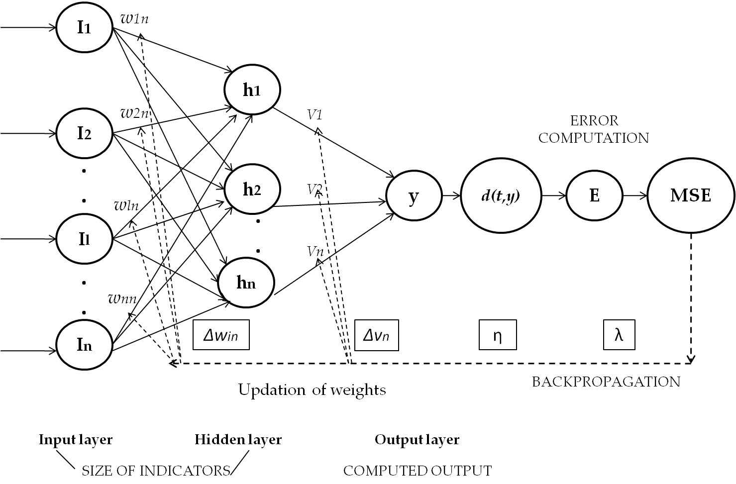Figure 1. The generic topology of the proposed MLFFNN model

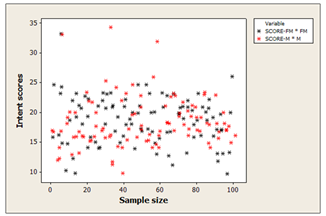Figure 2. The intent score distribution among males and females

The nature of data and its distribution have been examined. Table 2 shows the mean, standard deviation, variance and skewness of the indicators. It may be seen that the mean score is maximum for the indicator ‘APA’ and minimum for ‘CML’, which mean that the overall effects on ‘intent’ scoring is mostly contributed by ‘APA’ values. The indicator ‘I’ shows the most spread data distribution and so the highest variance. Among twenty, 15 indicators show positive skeweness (mean: 0.23, maximum: 0.92 for the case of ‘CML’). On the other hand, ‘APA’ presents the most negative skewness.

Reliability measure with Cronbach’s alpha shows the alpha value as 0.798, which is significant [22].

4.2. Data Analysis

Under this section, the results of the following experiments have been displayed.

1) ANOVA (refers to table 3)

2) Main effect of each indicator on the SCORE (could be seen in Fig.3)

3) MLR (could be seen in table 4, equation 6, and Fig.4)

4) PCA (refers to table 5 and Fig.5), and

5) Performances of the MLFFNNs (could be seen in table 6).

4.2.1. The Analysis of Variance (ANOVA)

ANOVA has been performed to test whether the groups of indicators are same or different from each other. Table 3 has shown the ANOVA result. In this table the ‘F’ statistics denotes a ratio of inter group variation and intra group variation. Therefore, a larger ‘F’ statistics value indicates higher inter group and intra group variations. Here, the ‘p’ value less than 0.05 supports that the experimental model is statistically significant.

Table 3. Descriptive statistics of the ‘intent’ data Indicator Mean Std. deviation Variance Skewness I 0.9453 0.8258 0.6820 0.10 T 1.0000 0.7810 0.6100 0.00 PADI 0.8408 0.7775 0.6045 0.29 AH 0.9453 0.7430 0.5520 0.09 FAD 0.9403 0.7978 0.6364 0.11 APA 1.2388 0.6875 0.4727 -0.35 SN 0.8856 0.8011 0.6418 0.21 OCI 0.9950 0.6189 0.3830 -0.03 AP 0.6119 0.7607 0.5787 0.79 EF 0.8905 0.5727 0.3280 -0.01 CML 0.5473 0.7134 0.5090 0.92 SA 1.0846 0.7796 0.6078 -0.15 ATLD 0.9801 0.7743 0.5996 0.03 CMR 0.8856 0.7084 0.5018 0.17 DP 1.1493 0.7600 0.5776 -0.26 RA 0.9154 0.7535 0.5678 0.14 VD 0.8507 0.7332 0.5376 0.12 NPA 0.9303 0.7517 0.5651 0.23 RAA 0.8607 0.7352 0.5405 0.01 RDA 1.0448 0.7516 0.5650 0.24

Table 4. ANOVA result Source DF SS MS F P Regression 20 498.66 24.93 1.61 0.049 Residual error 180 2795.23 15.53 Total 200 3293.89

4.2.2. The Main Effect Plots

The main effect plot shows the average outcome for each value of each indicator, combining the effects of the other indicators if and only if all indicators are independent. From ANOVA, it is seen that there is a considerable difference within and between groups, hence main effect plots could be useful to note the influence of the average scoring of the indicators on ‘intent’ assessment. In figure 3, the mean score is plotted against the value of the indicators.

In this figure the term ‘SCORE’ denotes the suicidal ‘intent’ score. In these plots it may be observed that for indicator ‘I’, the score ‘2’ averages of the most, while ‘0’ is the lowest and ‘1’ in between to influence the overall scoring of suicidal ‘intents’ for this dataset. Table 4 shows the summary of the average score loading/effects on ‘intent’ scoring. For this case 50% of the indicators have highest average score loading of ‘2’, while scores ‘0’ and ‘1’ contribute 25% each.

4.2.3. Multiple Linear Regressions

Multiple linear regressions have then been performed to mine the effects of the indicators (i.e. independent factors) on the ‘intent’ score (i.e. dependent factor). The regression equation is shown in equation 6.

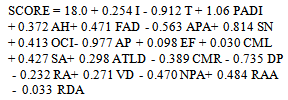(6)

The constants and the coefficients obtained through regressions are then used to validate the model with the test data (30% of the sample). Regression results are then compared with MLFFNNs and the human experts (see table 7).

Significant indicators are then extracted with the help of paired-t-test. Table 5 shows the significant indicators, such as ‘T’, ‘PADI’, ‘SN’, and ‘AP’ with p-values <0.05 (CI 95%).

Table 5. The main effect scores for the intent Indicator Average effect score loading I 2 T 0 PADI 2 AH 2 FAD 2 APA 0 SN 2 OCI 0 AP 1 EF 2 CML 1 SA 2 ATLD 2 CMR 1 DP 0 RA 1 VD 2 NPA 1 RAA 2 RDA 0

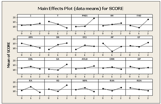Figure 3. Main effect plots (data mean) for the ‘intent’ score

The residual plots for the intent score could be seen in figure 3, which is a four-in-one plot to have a more concise view of the model. The top left and right plots show that the residuals (i.e. the deviations of the observed responses from the predicted responses) are normally distributed across the normality line. However, deviations could be noted for four cases having values higher than +10. The shape of the histogram plot resembles a normal probability distribution.

4.2.4. Principal Component Analysis

After obtaining the measures on the observed indicators PCA has been conducted for extracting more number of significant indicators that would account for the most of the variance in the observed indicators. It is performed using Minitab 14. One aim of this study is also to reduce the number of indicators based on the principal/significant indicators. Principal components are linear combinations of optimally-weighted observed indicators. Table 6 has shown the corresponding ‘proportion’ and ‘cumulative’ values. The term ‘Proportion’ denotes how much percentage of variance a variable has in the data. For example, ‘I’ accounts for 12.4% of variance in the data.

Table 6. The regression result: significant indicators Indicator Mean Std. deviations t-value p-value T 0.6119 0.7607 -2.34 0.020 PADI 0.8408 0.7775 2.64 0.009 SN 0.8856 0.8011 2.10 0.037 AP 1.0000 0.7810 -2.09 0.038

Figure 4 is the Scree plot showing the Eigen values of all the indicators. It corroborates that ‘I’, ‘T’, ‘PADI’, and ‘AH’ possess high Eigen values and the fall is quite steep. Then the fall in Eigene values is monotonically gradual. Hence, ‘I’, ‘T’, ‘PADI’, and ‘AH’ are taken as significant indicators.

Therefore, finally there are total six indicators such as ‘I’, ‘T’, ‘PADI’, ‘AH’, ‘SN’ and ‘AP’ which are chosen to develop the MLFFNN-3.

4.3. Results of the Performances of MLFFNN-1, 2 and 3

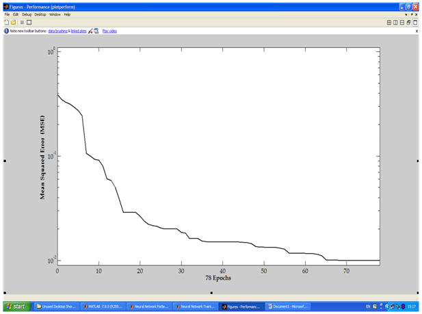
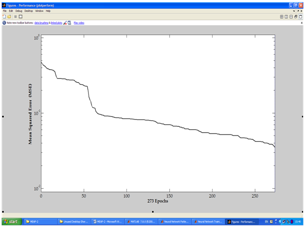
Performances of all the nets have been tested on a P-IV (Intel dual core) computer with 2 GB RAM and 3.0 GHz processor speed and compared among themselves and ten other human experts (mean experience 4.3 years). The performance results are shown in table 7 and figures 5 to 7 as follows. From the table is could be seen that the MSEs are negligible for all the neural nets and it is lowest for the MLFFNN-1 (MSE = 0.005). Due to higher number of indicators (i.e. 20), MLFFNN-2 converges early at the 78^th iteration at 0.02 sec. The converse could be seen with MLFFNN-3. Best learning rates of all the MLFFNN have been selected through careful parametric studies with all the nets. In a nutshell, MLFFNN-1 performs the best in terms of accuracy among all MLFFNNs.

Table 7. Eigen analysis results Indicator Eigen value (variance) Proportion Cumulative I 2.4706 0.124 0.124 T 2.2569 0.113 0.236 PADI 1.9313 0.097 0.333 AH 1.5473 0.077 0.410

While comparing with the interpretations given by ten human experts, it is seen that the average time taken to complete one full task with 15 indicators is around 15 minutes. It is 25 minutes and 10 minutes with 20 and 6 indicators. The MSE are 5% with 15 and 20 indicators. MSE increases with six indicators probably due to less number of information.

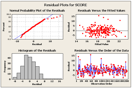Figure 4. Residual plots for the intent ‘score

Figure 5. Scree plot showing the indicators and the corresponding Eigen values

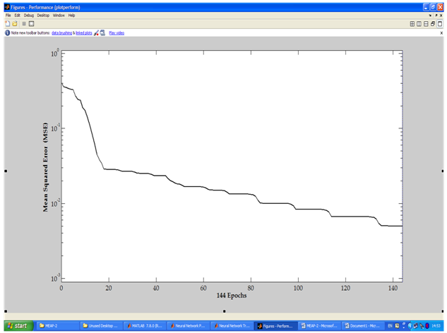Figure 6. Performance plot of MLFFNN-1

Figure 7. Performance plot of MLFFNN-2

Table 8. Performance measures of MLFFNNs and Human experts Items Regressions MLFFNN-1 MLFFNN-2 MLFFNN-3 Human experts (average performance) No. of indicators 15 20 06 15 20 06 15 20 06 No. of iterations - - - 144 78 273 - - - Execution time (sec) - - - 0.05 0.02 0.07 720 900 200 Gradient - - - 7.86e-07 5.53e-07 6.65e-07 - - - Best η - - - 0.01 0.02 0.05 - - - MSE 0.15 0.1 0.25 0.005 0.01 0.03 0.05 0.05 0.1

5. Conclusions and Future Scopes

The study draws the following conclusions.

● The collected suicidal intent data is reliable (Cronbach’s alpha = 0.798)[22].

● The attributes (i.e. BSIS indicators) are independent of each other as shown in the results of ANOVA (F-statistics 1.61).

● The main effect plot (refer to table 4 and figure 2) shows that the mean scores of 50% of the indicators are the highest, i.e. ‘2’ and accordingly influence the final ‘intent’ scoring in this dataset.

● By MLR and PCA, total six indicators such as ‘I’, ‘T’, ‘PADI’, ‘AH’, ‘SN’ and ‘AP’ are found statistically significant (i.e., considered as the quality indicators) in influencing the final intent scoring. It corroborates with the earlier results obtained through factor analysis[29][30]. These are used to design and develop the MLFFNN-3.

● With multiple linear regressions the best prediction could be possible with 15 indicators (MSE of 15%).

● MLFFNNs have outperformed the regressions- based predictions and predictions made by the human experts and the regressions analysis in terms of accuracy and speed.

● MLFFNN-1 (having 15 BSIS indicators) is technically most accurate (MSE = 0.005), i.e., only one misclassification (the 121^st case, which is originally having class label of ‘medium’ risk but classified under ‘mild’ risk). This observation is able to explain why 15 indicators are conventionally used in ‘intent’ scoring in the real-life. MLFFNN-2 and MLFFNN-3 misclassify 2 and 6 cases, respectively.

Figure 8. Performance plot of MLFFNN-3

● MLFFNN-2 (having all 20 BSIS indicators) having the most information converges with minimum number of iterations (i.e., 78) and hence at minimum time (i.e., 0.02 sec).

● The opposite picture is seen in case of MLFFNN-3 having the least number of information and hence taking more time (i.e. 0.07 sec) and iterations (i.e. 273) to converge.

The contribution of the paper lies on (i) systematic collection of ‘intent’ data from the real-life subjects and its analysis and (ii) designing and developing the neural networks to model the complete information of BSIS to map the way doctors make the scoring using their medical knowledge and logic.

The extension of this work could be the development of a complete GUI for its practical deployment in the clinics for the doctors to use as an assistive tool. Also the MLFFNNs could be trained with different datasets to enrich its maturity and robustness. However, the GUI-based tool has to be standardized prior its deployment.

ACKNOWLEDGEMENTS

The author gratefully acknowledges the help and support of the psychologists and psychiatrists during the data collection process.