-
Paper Information
- Next Paper
- Previous Paper
- Paper Submission
-
Journal Information
- About This Journal
- Editorial Board
- Current Issue
- Archive
- Author Guidelines
- Contact Us
American Journal of Biomedical Engineering
p-ISSN: 2163-1050 e-ISSN: 2163-1077
2012; 2(3): 131-135
doi: 10.5923/j.ajbe.20120203.07
Left Ventricle Segmentation in Cardiac MRI Images
 Abstract
 Reference
 Full-Text PDF
 Full-Text HTML
Marwa M. A. Hadhoud1, 2, Mohamed I. Eladawy3, Ahmed Farag1, Franco M. Montevecchi2, Umberto Morbiducci2
1Department of Biomedical Engineering, Faculty of Engineering, Helwan University, Cairo, Egypt
2Department of Mechanics, Politecnico di Torino, Torino, Italy
3Department of Communication & Electronics, Faculty of Engineering, Helwan University, Cairo, Egypt
Correspondence to: Marwa M. A. Hadhoud, Department of Biomedical Engineering, Faculty of Engineering, Helwan University, Cairo, Egypt.
| Email: |  |
Copyright © 2012 Scientific & Academic Publishing. All Rights Reserved.
Imaging of the left ventricle using cine short-axis MRI sequences, considered as an important tool that used for evaluating cardiac function by calculating different cardiac parameters. The manual segmentation of the left ventricle in all image sequences takes a lot of time, and therefore the automatic segmentation of the left ventricle is main step in cardiac function evaluation. In this paper, we proposed an automatic method for segmenting the left ventricle in cardiac MRI images. We applied pixel classification method by using number of features and KNN classifier for segmenting the left ventricle Cavity, and from its output we can get the endocardial contour. Then, we transformed image pixels from Cartesian to polar coordinates for segmenting the epicardial contour. This method was tested on large number of images, and we achieved good results reached to 95.61% sensitivity, and 98.9% specificity for endocardium segmentation, and 93.32% sensitivity, and 98.49% specificity for epicardium segmentation. The results of the proposed method show the availability for fast and reliable segmentation of the left ventricle.
Keywords: Cardiac MRI, Segmentation, Pixel Classification
Article Outline
1. Introduction
- Cardiovascular diseases cause 17.5 million deaths every year in the world[1]. The early diagnosis of the cardiovascular diseases plays an important role in the recovery.Cardiac MRI imaging using cine MRI sequences, considered as an important tool that used for evaluating cardiac function. Evaluation of cardiac function requires calculation of different cardiac parameters (i.e. ejection fraction (EF), left ventricle mass (LVM), left ventricle volume, wall thickness, or wall thickening). All of these parameters depend on segmenting the endocardial, and epicardial contours of the left ventricle from the image sequences that are acquired from cardiac imaging technique. The manual segmentation of these contours from all dataset (i.e. all time frames per all slices) takes a lot of time and effort from the cardiologist. Therefore, the automatic segmentation is very important, and can be considered as a challenging task.In the short-axis MRI image, the blood pools (i.e. of the right and left ventricle) appear bright and all their surrounding structures appear dark (i.e. myocardium, lung, and liver) with different intensities, as shown in fig. 1. Also the left ventricle looks like a circular in the short-axis image.There are several techniques used in the left ventricle segmentation. Collections of these techniques are reviewedin[2,3]. In general, we can classify these techniques according to the algorithm that used in the segmentation process to, image-based methods (i.e. which include thresholding, region growing, … etc)[4-6], pixel classification methods (i.e. using clustering, and classification methods)[7-9], deformable models (i.e. like active contour model)[10,11], model-based methods (i.e. active shape model (ASM), and active appearance model (AAM))[12,13], and finally the atlas guided method[14,15].In this paper, we concentrate on the pixel classification technique. Image segmentation by using this technique, partitioning the image to regions by classifying the pixels to different classes according to their features. The classification part is done by using supervised or unsupervised algorithms. Usually in the cardiac segmentation, the features used are the gray level intensities, and the classification is done by clustering methods, or Gaussian Mixture Model (GMM).Pednekar et al. in[7], used the localization of the heart as an initial step to estimate the LV region, which used to get the intensity statistics for the LV blood and myocardium by using Expectation-Minimization (EM) algorithm that followed by Gaussian Mixture learning step.Lynch et al. in[8], used the diffusion-based filter to smooth the cardiac images while maintaining the important edges information. Then he used the k-means clustering algorithm. From the resulting labels, the LV cavity is detected by using the approximation to a circle, and the closest region to a circle considered as the LV cavity. Then the closest blood pool to the LV cavity is the RV blood pool, which help to know the thickness of the myocardium that used for segmenting the epicardium.Gering in[16], used a new contextual dependency network (CDN) in the cardiac segmentation. This network doing classification in different stages. In the beginning, the pixels classified by using EM algorithm, then used a Markov random field to take into consideration the neighbourhood interaction between pixels, then take the region properties and relationship between regions to complete the segmentation process.This paper is structured as follows. The next section presents the localization method of the region of interest (ROI) from cardiac MRI images to reduce the working area, because the cardiac MRI image contains a lot of structures in it. The third section will be focus on the segmentation of the left ventricle which consists of two main steps. It starts with segmenting the endocardium area, and then ends with segmenting the epicardium area. The segmentation of the endocardium depends on a pixel classification method that extracts different features from the dataset (i.e. gradient magnitude, largest eigenvalue, output of median filter, and the gray value) and uses the KNN in the classification of the target object. The segmentation of the epicardium contour depends on transforming the ROI from Cartesian to polar coordinates, and using the results of the endocardium segmentation as a mask to remove unwanted edges to achieve our goal of segmenting the epicardium contour.
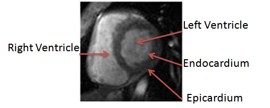 | Figure 1. Left ventricle in a short-axis MRI image |
2. Localization of the Cardiac
- For localizing the general position of the heart in cardiac MRI images, we applied the algorithm mentioned in[17]. This algorithm depends on calculating the standard deviation between all images for different time frames in the middle slice, to compute the standard deviation map, that used to determine the general position of the heart. The flowchart that describe the steps of this algorithm shown in fig. 2.As mentioned, to get the standard deviation map, we should determine the middle slice that we will work on it. This is because the cardiac has different views along the long-axis (i.e. from apex to base), as shown in fig. 3. In the middle slice, we can see the left ventricle as a circular shape, so there will be a great standard deviation between the myocardium, and the blood pool, according to the movement of the heart.After getting the standard deviation map, this image is convereted to binary image. The threshold that used in binarization, is calculated after plotting the probability density function of the standard deviation values, and take the threshold value that gets 80% of the area under the probability density curve function.
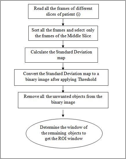 | Figure 2. Flowchart of the localization algorithm |
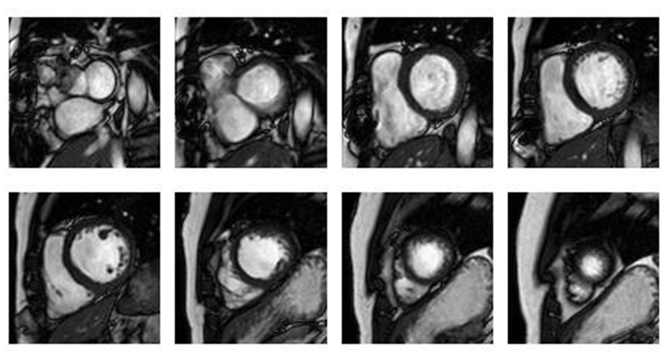 | Figure 3. Cardiac views at different slices along the long-axis |
3. Left Ventricle Segmentation
- As shown in fig. 1, segmenting the left ventricle depends on segmenting two different contours. The interior contour is called endocardium that surrounds the left ventricle blood pool, and the external contour that is called epicardium. There are some difficulties in segmenting these contours[3]. For segmenting the endocardium, there are some difficulties according to the presence of the papillary muscles and trabeculations inside the heart chamber, that has the same intensity of the myocardium. Also, there are some gray value inhomogeneities inside the left ventricle cavity itself. For the epicardium, the difficulties generated because around the epicardium there are different tissues (i.e. fat, and lung) that have different intensities, and there are poor contrast between these tissues and the myocardium. To segment these contours, we will begin in segmenting the endocardium because it is easier in segmentation due to the good contrast of the LV cavity and the myocardium. In the segmentation of the endocardium, we will applied the algorithm mentioned in[18]. After segmenting the endocardium, we will used the output of segmentation as a mask to help us in segmenting the epicardium.
3.1. Endocardium Segmentation
- The segmentation of the endocardium, depends on segmenting the LV cavity, by extracting different features (i.e. the gradient magnitude, the largest eigenvalue, the output of median filter, and the gray value) from each pixel in the image. Then, we apply the principal component analysis (PCA) to reduce the feature space dimension, and getting the final feature vector that used with the KNN classifier for segmenting the pixels to blood or not.This part of segmentation, needs a training stage to help in learning the classifier the main characteristics of each class. So, we applied our algorithm on 13 different patient[19]. We took randomly 20 images from each patient for training.During preparing the training dataset, we will need to label the LV cavity as class 1 and its surrounding area as class 2. So, we did that by using the manual segmentation of the inner contour that attached with the dataset.We chose the features (used in the segmentation) due to the nature of the LV cavity that we want to segment it. The LV cavity appears bright and the myocardium that surrounds it appears dark. So, we need to improve edges that surround the LV cavity. For that we chose to take the gradient magnitude, and the largest eigenvalue as features. We get the gradient magnitude, and the largest eigenvalue at different scales (i.e. 1,2,4,8,16) and take the maximum over all scales. Although the MRI provides high contrast between the blood and the myocardium, but there is gray inhomogeneites inside the LV cavity. Because of that we chose to take the output of applying the median filter as features, and we applied different window sizes (i.e. 3, 5, and 7), and took all these outputs as features. We took all of these features beside the gray value of the pixel itself.Although, we reduced the processing area on the image by determining the ROI. But still we have a lot of pixels in the training dataset that will be used as instances. To reduce the dimension of the training samples, we applied image patches technique that used in object recognition in images. Image patches are squared subimages extracted from an image. We applied image patches on training dataset un-overlaped, and on testing dataset overlapped to scan all pixels in the image.We took image patches for different reasons, the first one to reduce the training samples that will be used in the training stage. The second one because the patches divide the image to different subimages, so it will take the neighborhood characteristics of each pixel in describing the features of each subimage, and because of that it considered as local features.After applying patches, we reduced the training samples, but in the same time we increased the feature vector of each sample. We used 6 different features, and for each one we applied the patch technique with size (7X7). So, for each sample, we will have 72 components multiplied by the number of features. Therefore, we applied the principal component analysis (PCA) on the feature space to reduce its dimension. After applying PCA, we tested different numbers of the resulting components as features (i.e. 5, 10, ….., etc.) with the KNN classifier with K=1, and for each number of features we evaluate the output by different evaluation parameters, to choose which one is the best. The detection of the LV cavity from the output of the KNN classifier, will be done after doing post-processing stage to determine the most circular connected component in the image, because the LV cavity appears circular as mentioned before, and we did that by calculating the circularity of each connected component as Eq. 1, and chose the most circular object.
 | (1) |
3.2. Epicardium Segmentation
- There are different tissues (i.e. fat, lung, and liver) that surround the myocardium, and these tissues have different intensity values. Also, the part of the epicardium in front of the right ventricle is thin in thickness. All of these issues make the segmentation of the epicardium is difficult.For segmenting the epicardium, we convert the subimage (extracted from ROI image) that centered in the center of the left ventricle cavity, and its radius equal 30 pixels, from cartesian to polar coordinates. After getting the polar image of these pixels that cover this area, we apply Canny[20]edge detection on this image, to get polar edge map image. Also, we convert the same subimage of the binary image of the left ventricle cavity (resulted from the previous stage) to polar coordinates with the same center and for the same radius. Then we used this image as a binary mask (after inverting it) to delete all unwanted edges (i.e. inside left ventricle cavity, and endocardium too) from the polar edge map image to help us determining the edge map of the epicardium only.As we mentioned before of that, there are low contrast between myocardium and its surrounding tissues, this make small edges inside and outside the myocardium. For this reason, we deleted the small connected components in the edge map to reach to the edges that represent the epicardium contour at different parts.The first point at each column in the resulting image considered as edge point. After determining all the edge points, we inverse the transform of the edge points coordinates from polar to cartesian, then get the convex hull of these points, and get its boundary border that represent the epicardial contour.
4. Evaluation
- To evaluate our work, we calculate different parameters that used to measure the performance of the segmentation algorithm. These paramers are sensitivity, specificity, and dice metric. Beside these parameters we calculated the ejection fraction (EF), and compared its values from the automatic segmentation algorithm, and the manual segmentation by correlation analysis.
4.1. Sensitivity, and Specificity
- The sensitivity is the proportion of true positivies of the automatic segmentation output to the manual segmentation output (i.e. reference output).The specificity is the proportion of true negativies of the automatic segmentation output to the manual segmentation output.These parameters were calculated as in Eq. (2)
 | (2) |
4.2. Dice Metric
- The dice metric, DM, was calculated as in Eq. (3)
 | (3) |
5. Results
- The automatic method of segmenting the left ventricle was tested on 13 different patients (i.e. 3 different slices, 20 phases for each slice). The automatic segmentation results can be seen in Fig. 4. For the endocardium segmentation, we tested different number of features, the first 25 features give the highest accuracy.As shown in Table. 1, the average sensitivity , and specificity, for segmenting the endocardium area are 0.9561 ± 0.0625, and 0.9890 ± 0.0089. The segmentation of the epicardium area achieved 0.9332 ± 0.0766, and 0.9849 ± 0.0092 sensitivity, and specificity.We achieved good results by evaluating our algorithm by dice metric. It reached to 0.8937 ± 0.0747 for endocardium area segmentation, and 0.9161 ± 0.0473 for epicardium area segmentation.
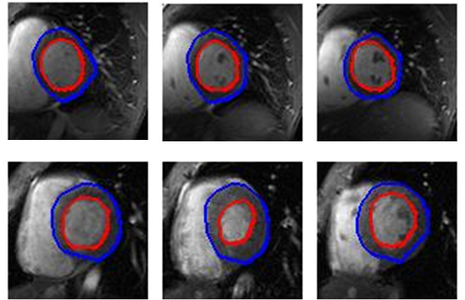 | Figure 4. Final results of automatic segmentation, the blue contour are the epicardium, and the red contour is the endocardium |
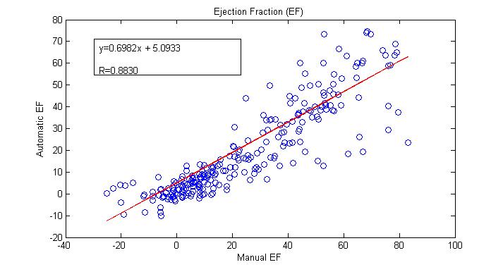 | Figure 5. Ejection fraction (EF) results compared between the automatic and manual calculation |
6. Conclusions
- Fully automatic algorithm for detecting and segmenting the left ventricle from cardiac MRI images was proposed in this paper. The algorithm used the standard deviation variations between different phases in a specific slice to localize the global position of the heart. The automatic segmentation method divided to two parts. The first part concentrated to segment the endocardium area by a pixel classification method, that depends on extracting different features (i.e. gradient magnitude, largest eigenvalue, output of median filter, and gray value) with the KNN classifier. The secod part concentrated to segment the epicardial area by tracing the edge points after converting image from cartesian to polar coordinates and deleting all edges of the endocardium by using the output of the first part to help us. The results of the proposed method show the availability for fast and reliable segmentation of the left ventricle.
ACKNOWLEDGEMENTS
- M. Hadhoud would like to thank Elissa Ficcara, and Santa Di Cataldo (Department of Control and Computer Engineering, Politecnico di Torino, Torino, Italy) for their help and advices during this research, also would like to thank organizers and responsible of FFEEBB program, because this program gives to her good chance to do part of her PhD research in Politecnico di Torino, and cooperates with her colleagues to do this research.
References
| [1] | World Health Organization of cardiovascular diseases, [online], www.who.int/cardiovascular_diseases/en. |
| [2] | J.S. Suri. Computer vision, pattern recognition and image processing in left ventricle segmentation: the last 50 years. Pattern Analysis and Applications, 3(3):209-242, 2000. |
| [3] | Caroline Petitjean, Jean-Nicolas Dacher, "A review of segmentation methods in short axis cardiac MR images", Medical Image Analysis 15, 2011, pp.169–184. |
| [4] | Katouzian, A., Konofagou, E., Prakash, A., 2006. A new automated technique for left and right-ventricular segmentation in magnetic resonance imaging. Conf. Proc. IEEE Eng. Med. Biol Soc. 1, 3074–3077. |
| [5] | Yeh, J., Fua, J., Wua, C., Lina, H., Chaib, J., 2005. Myocardial border detection by branch-and-bound dynamic programming in magnetic resonance images. Comput. Methods Programs Biomed. 79 (1), 19–29. |
| [6] | Cousty, J., Najman, L., Couprie, M., ClTment-Guinaudeau, S., Goissen, T., Garot, J., 2010. Segmentation of 4D cardiac MRI: automated method based on spatiotemporal watershed cuts. Image Vis. Comput. 28, 1229–1243. |
| [7] | Pednekar, A., Kurkure, U., Muthupillai, R., Flamm, S., 2006. Automated left ventricular segmentation in cardiac MRI. IEEE Trans. Biomed. Eng. 53 (7), 1425–1428. |
| [8] | Lynch, M., Ghita, O., Whelan, P., 2006. Automatic segmentation of the left ventricle cavity and myocardium in MRI data. Comput. Biol. Med. 36 (4), 389–407. |
| [9] | Stalidis, G., Maglaveras, N., Efstratiadis, S., Dimitriadis, A., Pappas, C., 2002. Modelbased processing scheme for quantitative 4-D cardiac MRI analysis. IEEE Trans. Inf. Technol. Biomed. 6 (1), 59–72. |
| [10] | Ranganath, S., 1995. Contour extraction from cardiac MRI studies using snakes. IEEE Trans. Med. Imag. 14 (2), 328–338. |
| [11] | Santarelli, M., Positano, V., Michelassi, C., Lombardi, M., Landini, L., 2003. Automated cardiac MR image segmentation: theory and measurement evaluation. Med. Eng. Phys. 25 (2), 149–159. |
| [12] | Mitchell, S., Lelieveldt, B., van der Geest, R., Bosch, J., Reiber, J., Sonka, M., 2001. Multistage hybrid active appearance model matching: segmentation of left and right ventricles in cardiac MR images. IEEE Trans. Med. Imag. 20 (5), 415– 423. |
| [13] | Zambal, S., Hladuvka, J., Bühler, K., 2006. Improving segmentation of the left ventricle using a two-component statistical model. In: Proceedings of Medical Image Computing and Computer-Assisted Intervention (MICCAI). LNCS, pp. 151–158. |
| [14] | Lorenzo-Valdés, M., Sanchez-Ortiz, G., Mohiaddin, R., Rueckert, D., 2002. Atlas-based segmentation and tracking of 3D cardiac MR images using non-rigid registration. In: Proceedings of Medical Image Computing and Computer- Assisted Intervention (MICCAI). LNCS, Tokyo, Japan, pp. 642–650. |
| [15] | Zhuang, X., Hawkes, D., Crum, W., Boubertakh, R., Uribe, S., Atkinson, D., Batchelor, P., Schaeffter, T., Razavi, R., Hill, D., 2008. Robust registration between cardiac MRI images and atlas for segmentation propagation. In: Society of Photo-Optical Instrumentation Engineers (SPIE) Conference, p. 691408. |
| [16] | Gering, D., 2003. Automatic segmentation of cardiac MRI. In: Proceedings of Medical Image Computing and Computer-Assisted Intervention (MICCAI). LNCS, vol. 1, pp. 524–532. |
| [17] | M. Hadhoud, M. Eladawy, A. Farag, " Automatic Global Localization of The Heart From Cine MRI images", 2011 IEEE International Symposium on IT in Medicine & Education ( ITME), 2011, pp. 35-38. |
| [18] | M. Hadhoud, M. Eladawy, A. Farag, “Left Ventricle Cavity Segmentation from Cardiac Cine MRI ", accepted in International Journal of Computer Science Issues (IJCSI), March 2012, Vol. 2, pp. 398-402. |
| [19] | Cardiac MRI Dataset, [online],http://www.cse.yorku.ca/~mridataset/. |
| [20] | R. C. Gonzalez, and R. E. Woods, “Digital Image Processing”, Upper Saddle River, New Jersy: Prentice-Hall, 2002. |