-
Paper Information
- Next Paper
- Previous Paper
- Paper Submission
-
Journal Information
- About This Journal
- Editorial Board
- Current Issue
- Archive
- Author Guidelines
- Contact Us
American Journal of Biomedical Engineering
p-ISSN: 2163-1050 e-ISSN: 2163-1077
2012; 2(3): 124-130
doi: 10.5923/j.ajbe.20120203.06
Analysis of Cerebral Infarct Signal Intensity on Diffusion-Weighted MR Images Using Frequency Domain Techniques
 Abstract
 Reference
 Full-Text PDF
 Full-Text HTML
S. S. Shanbhag1, G. R. Udupi2, K. M. Patil3, K. Ranganath4
1Electronics and Communication Engineering, Gogte Institute of Technology, Belgaum, 590001, India
2Vishwanathrao Deshpande Rural Institute of Technology, Haliyal, 581329, India
3Retired, Indian Institute of Technology (Madras), Belgaum, 590009, India
4RAGAVS, Diagnostics and Research Center Pvt Ltd, Bangalore, 560011, India
Correspondence to: S. S. Shanbhag, Electronics and Communication Engineering, Gogte Institute of Technology, Belgaum, 590001, India.
| Email: |  |
Copyright © 2012 Scientific & Academic Publishing. All Rights Reserved.
Early and accurate diagnosis of cerebral infarction plays a vital role in the implementation of successful treatment and thereby improving the quality of life. Diffusion Weighted Magnetic Resonance Imaging (DW-MRI) is a highly sensitive tool for the detection of early changes in the water diffusion that characterizes various brain pathologies, largely, cerebral infarctions. Studies were performed on a set of Diffusion Weighted (DW) images of the human brain (in the axial plane) to find the relationship between the light intensity High Frequency Power (HFP) values and the time course of cerebral infarction, and to present evidence in defining the stages of cerebral infarction. Analysis of the results show that the difference in the light intensity HFP values on the DW images for the subjects with cerebral infarction compared to their contralateral normal hemisphere, were highly significant (p < 0.01) in the areas of the brain, where there was a high incidence of infarction. The relative increase in the light intensity HFP values (RHFP) for the subjects with cerebral infarction were in the range of (153.06 – 1780.43) times compared to their corresponding HFP values on the contralateral normal hemisphere. The observed RHFP values increased progressively with time and were at the peak for the examinations between 1 to 4 days and thereafter reduced to reach the minimum after 15 days. There was a negative correlation (r = - 0.74) observed between the RHFP values and the time stage of cerebral infarction. The evolution of the RHFP values observed subsequent to infarction is suggestive that they can be supportive in understanding the developmental stages of infarction and can be helpful in predicting the stage of infarction. The quantitative changes in the light intensity HFP values can be assessed to derive information about the early changes taking place in the brain tissue. Further their adoption in clinical diagnosis and treatment of cerebral infarction could be helpful and informative. In conclusion, the proposed method could positively assist the neuro-surgeons for speedy diagnosis and execution of treatment to protect the subjects from additional damage to their brain tissue. In summary, the present study provides evidence that the light intensity HFP values on the DW images in the region of cerebral infarction can be used to markedly distinguish the infarct subjects quantitatively from the normal subjects. The relative increase in the light intensity HFP values on the DW images for the subjects with cerebral infarction were in the range of (153.06 – 1780.43) times compared to their corresponding HFP values on the contralateral normal hemisphere. The quantitative changes in the values of the light intensity HFP parameter on the DW images can be assessed and positively employed to provide useful information about the early changes taking place in the brain tissue and can be helpful in determining the stage of cerebral infarction. Therefore the adoption of the proposed quantitative method in the clinical diagnosis and treatment of cerebral infarction could be helpful and instructive.
Keywords: Diffusion Weighted Imaging, High Frequency Power, Infarct, Magnetic Resonance Imaging, Signal Intensity
Article Outline
1. Introduction
- Cerebral infarction is a leading cause of death and a major cause of long term disability. Post infarction treatments offered mainly depend on the timing after infarction to determine the stages of brain damage[1]. Recently, Diffusion Weighted Magnetic Resonance Imaging (DW-MRI), an imaging technique based on the sensitivity of magneticresonance to microscopic mobility of water molecules within tissues, has emerged to be applicable in the clinical diagnosis and treatment of cerebral infarction[2-4]. DW-MRI is considered to be the most sensitive tool for the diagnosis ofearly cerebral infarction, mainly because of its exquisite sensitivity in the detection of early changes in the water diffusion that characterizes infarction[5]. While it takes hours to reach the diagnosis with conventional Magnetic Resonance Imaging (MRI), DW-MRI allows for the detection of cerebral infarcts within minutes after its onset and in addition provides clinically valuable information about the age of infarction[6-8]. Investigators from several previously published studies have described temporal evolution of the Apparent Diffusion Coefficient (ADC) values within lesions following cerebral infarction, to identify their usefulness in the clinical diagnosis of the progress of infarction and treatment. The ADC values reported from these studies have been computed from a single axial section (showing infarction) on the Diffusion Weighted (DW) images. Also the calculation of the ADC values considers only a small region within the infarcted area and further different studies propose diverse methods for calculating the ADC values[9-12]. Additionally, since the ADC values vary spatially within the infarcted area, a comprehensive understanding of the entire infarcted area would be necessary for better analysis[13-16].In contrast to the available work concerning cerebral infarction using ADC values, the temporal evolution of infarct signal intensity on the DW images is less well documented in the literature[1, 17, 18]. Furthermore radiologists in a variety of clinical settings depend only on the DW images (signal intensity variations) to review subjects with cerebral infarctions. In this direction if the progression of the signal intensity on the DW images following cerebral infarction can be quantified and assessed, this information would surely aid the radiologists in early and accurate diagnosis of infarction. This would result in subjects receiving prompt treatment, which, in turn, improves their chances of survival and recovery. Therefore the objective of the present work is to determine the role of signal intensity changes on the DW images of the human brain in the axial plane in the early diagnosis and classification of the stages of cerebral infarction. Mainly an effort is made in grading the signal intensity changes on the DW images using the light intensity High Frequency Power (HFP) values. The new method proposed in the present work takes care of the drawbacks listed earlier for the studies carried out in the past using ADC values for the diagnosis of cerebral infarction. In the proposed method all the axial sections showing cerebral infarction are taken into account and also the entire infarcted area on each axial section is considered to evaluate the light intensity HFP values. Therefore the method assures that there is no loss of information as it covers larger area of the brain and also expertise is not essential as the entire infarcted area is considered for carrying out the investigation. The light intensity HFP values obtained from the infarct subjects are compared to their corresponding HFP values from the contralateral normal hemisphere for the same subject to find the relative changes in the HFP values. The relative changes in the HFP values so obtained are employed to realize a quantitative model for the time course of the infarct signal intensity variations. The method could positively aid in the speedy and accurate radiological diagnosis of the infarct subjects and additionally provide important reference in judging the timing and developmental stages of cerebral infarction.
2. Methods
- DW-MRI is a well-established clinical tool that provides unique information on the viability of the brain tissue. This sequence produces MRI based quantitative maps of the microscopic, natural displacements of water molecules that occur in the brain tissues as a part of the physical diffusion process. Water molecules are used as probes that reveal microscopic details about the architecture of both healthy and unhealthy brain tissues[19, 20]. The rate of water diffusion in the brain tissue is a direct function of its physiological state, and impacted by brain pathologies, such as cerebral infarction. There is an increased restriction to water mobility observed in the area of infarction within the brain tissue, and this produces a bright imaging appearance in the area of cerebral infarction when compared to the other healthy areas of the brain tissue[21]. The observed signal intensity peaks in 3 - 4 days and may be persistently high as long as 14 days after the onset of infarction. Signal intensity further decreases with time and reverts to normal by the end of the second week[18]. Accordingly detection of the areas of the brain with high signal intensity variations on the DW images subsequent to infarction, may allow for the evaluation of the affected area and further quantification of the observed signal intensity may prove to be useful in the early diagnosis and characterization of the different stages of cerebral infarction.
2.1. Diffusion Imaging Protocol and Clinical Data
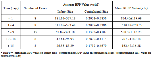
- All the subjects underwent clinical MR imaging with 1.5 T symphony maestro class MR scanning system from Siemens. DW imaging was performed by using a multisection, single-shot, spin-echo, echo-planar pulse sequence with following parameters: TR = 3200 ms, TE = 94 ms, acquisition matrix = 128 x 128, FOV = 230 mm x 230 mm, and diffusion gradient value of b = 1000 s/m2 along 19 axial sections, 5 mm thick section and intersection gap of 1.5 mm.For the purpose of our study 40 cases (31 male, 09 female, ages 29 – 93 years with an average of age of 66 years) of cerebral infarction were diagnosed and verified with radiology data. MRI and DW imaging examinations were performed on eight subjects within 24 hours of symptom onset; eight subjects between days 1 and 4; fifteen subjects between days 5 and 9; six subjects between days 10 and 14; and three subjects after day 15. For all the subjects with cerebral infarction considered, we confirmed the appearance of infarction by ruling out the possibility of bright intensity due to T2 shine through effects. This was done by verifying the appearance of hyperintensities on DW images and concomitant-reduced ADCs relative to the contralateral normal brain in their initial MRI studies. The ethics approval was obtained from the committee of clinical research at the RAGAVS diagnostic and Research center, Bangalore, India, and Vikram Hospital, Bangalore, India.
2.2. Light Intensity High Frequency Power
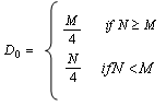
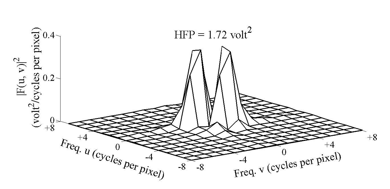
- DW-MRI makes it to visualize and measure the altered rates of water diffusion, by producing a bright imaging appearance in the area of cerebral infarction. Consequently on examining the spatial intensity variation distribution on the DW images for the subjects with cerebral infarction, it is observed that the light signal intensity is not uniformly distributed over the entire DW image. There are abrupt jumps in the light signal intensity in the area of infarction in contrast to the other healthy areas of the brain where the light signal intensity distribution is almost uniform. Exploring the power spectrum of the DW intensity image for the subject with cerebral infarction would thereby result in a higher value for the higher spatial frequency power component out of the total power spectrum, in the area of infarction, when compared to the higher spatial frequency power component on the contralateral normal (healthy) hemisphere (mirror image) for the same subject. Consequently the light intensity HFP value in the area of infarction is much elevated when compared to the light intensity HFP value on the contralateral normal hemisphere for the same subject. The relative light intensity HFP values[RHFP = (maximum HFP value on infarct side - corresponding HFP value on contralateral side) / corresponding HFP value on contralateral side] are quantified across different subjects diagnosed with cerebral infarction and are employed in differentiating infarct tissues from healthy tissues and further used in the categorization of the different stages of cerebral infarction.
2.3. Image Analysis
- The DW images obtained in DICOM format are converted to bmp format with intensities scaled to fit the conventional range of (0–255). This is done to reduce the complexity in the image manipulation algorithms and to achieve speed up in processing the images. The DW image obtained from the subject in the axial plane is divided into six anatomically significant areas as shown in Figure 1.
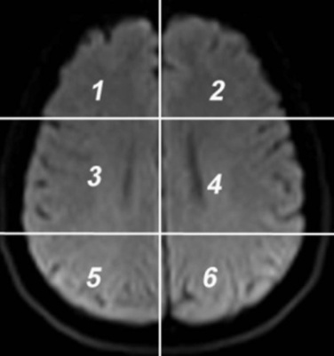 | Figure 1. Axial DW image showing areas |
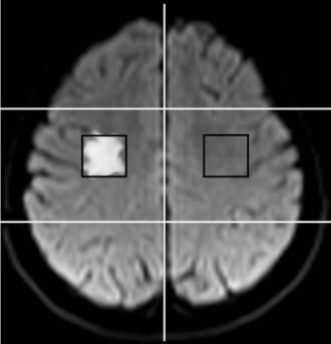 | Figure 2. Axial DW image showing ROI on the infarct side (area 3, axial section 10) and contralateral normal hemisphere |
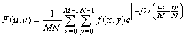 | (1) |
 | (2) |
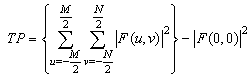
 | (3) |
 | (4) |
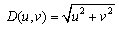
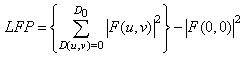
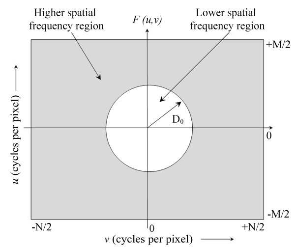 | Figure 3. The Fourier spectrum, F (u, v), of an image showing the higher and lower spatial frequency regions |
 | (5) |
 | (6) |
3. Results and Discussions
- The DW image for a subject showing infarction in area 3 and at axial section 8 is shown in Figure 4.
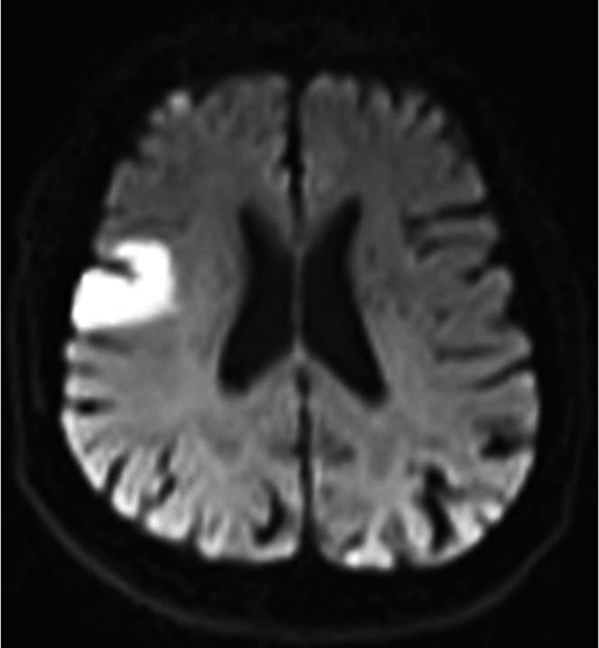 | Figure 4. Axial DW image showing infarction in area 3 |
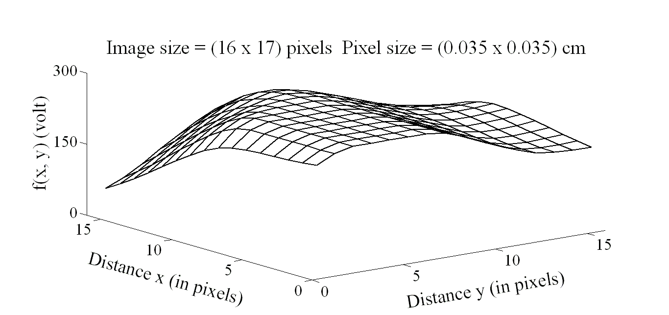 | Figure 5. Image intensity distribution for the subject with infarct in area 3 |
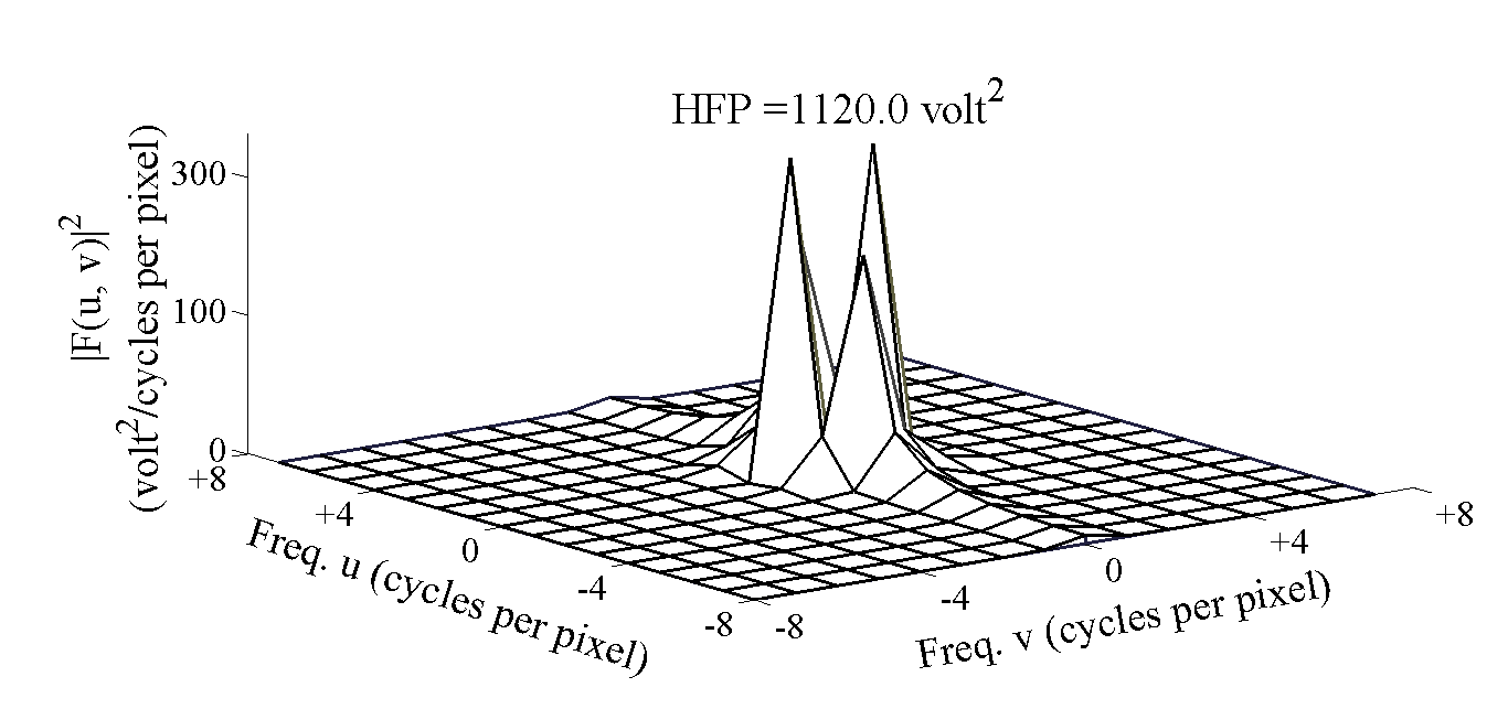 | Figure 6. Power spectrum for the subject with infarct in area 3 |
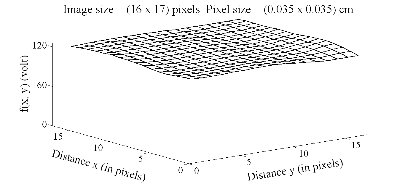 | Figure 7. Image intensity distribution on the contralateral hemisphere |
 | Figure 8. Power spectrum on the contralateral hemisphere |
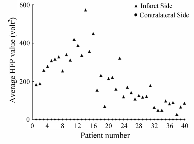 | Figure 9. Variation in the average HFP values for the infarct subjects with the corresponding average HFP values from the contralateral hemisphere |
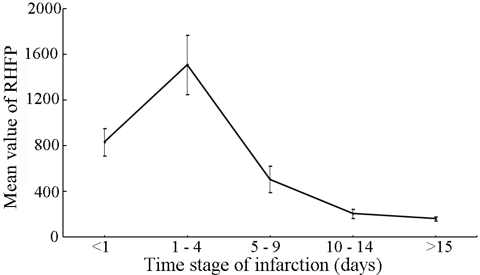 | Figure 10. Variation in the mean RHFP values with the time stage of cerebral infarction |
|
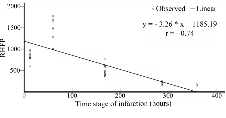 | Figure 11. Variation in the RHFP values with the time stage of cerebral infarction |
4. Conclusions
ACKNOWLEDGEMENTS
- The authors would like to thank Dr. Sudhir Pai (Sr. Consultant, Neurosurgeon, Vikram Hospital, Bangalore, India) for assistance in data collection and Dr. Deepak Y. S. (D.N.B. Resident, RAGAVS Diagnostic and Research Center, Bangalore, India) for his valuable comments and suggestions.