Seyed Navid Resalat , Seyed Kamaledin Setarehdan
Control and Intelligent Processing Center of Excellence, School of Electrical and Computer Engineering, College of Engineering, University of Tehran, Tehran, Iran
Correspondence to: Seyed Kamaledin Setarehdan , Control and Intelligent Processing Center of Excellence, School of Electrical and Computer Engineering, College of Engineering, University of Tehran, Tehran, Iran.
| Email: |  |
Copyright © 2012 Scientific & Academic Publishing. All Rights Reserved.
Abstract
Brain Computer Interfacing (BCI) systems, which are a new communicating channel between humans and the computers are growing rapidly. One such a method is based on the Steady State Visual Evoked Potentials (SSVEP), which can be recorded during visual stimulating of the subject by a twinkling light source with a fixed frequency. An important parameter to be considered is the effect of the inter-sources distance on the accuracy of such BCI systems. In particular inter-sources (LEDs) distances of 4, 14, 24, 44 and 64 cm when the sources plane is located 60 cm away from the subject's eyes (producing inter-sources visual angles of 3.8°, 13.4°, 22.6°, 40.2° and 56° respectively) were examined. In addition, four different sweep lengths of 0.5, 1, 2 and 3 seconds are considered. In addition, due to the usage of the AR models for feature extraction from the SSVEP signals, selection of the best AR model together with the best classifier among the LDA, the SVM and the Naïve Bayes are studied. It is showed that the BCI system with D=44 cm, AR order of 13 and either the LDA or the SVM classifiers could produce the best results compared to the other cases.
Keywords:
Brain Computer interface (BCI), Steady State Visual Evoked Potential (SSVEP), Inter-sources distance, Auto regressive model, Information Transfer Rate (ITR)
Cite this paper:
Seyed Navid Resalat , Seyed Kamaledin Setarehdan , "A Study on the Effect of the Inter-Sources Distance on the Performance of the SSVEP-Based BCI Systems", American Journal of Biomedical Engineering, Vol. 2 No. 1, 2012, pp. 24-31. doi: 10.5923/j.ajbe.20120201.04.
1. Introduction
Using the EEG signal as a communication channel was first proposed by Hans Berger in 1929[1]. The first Brain Computer Interfacing (BCI) system was however designed in Dr. Vidal’s laboratory in 1973[2]. Various BCI systems were then developed and used with different levels of success. One such a method is developed based on the visual evoked potentials (VEPs)[3]. Based on the kind of the visual stimulation used, these signals can be divided into three main modes of Pattern Reversal (PR), Pattern Onset/Offset (PO) and Flash (F)[3]. Pattern Reversal Visual Evoked Potentials (PRVEPs) is generated when an external light source with a constant twinkling frequency provoke the visual system[4]. When the twinkling frequency is below 6 Hz, the resulting potentials are known as Transient VEPs (TVEPs) otherwise they are called Steady State VEPs (SSVEPs)[5-6]. Previous studies have shown that these signals can be effectively recorded at the occipital lobe of the brain having the same fundamental frequency of the twinkling light source together with its 2’nd and occasionally 3’rd harmonics[6-8]. By providing multiple light sources with different twinkling frequencies to the subject, it will be possible to produce amulti-channel BCI system by determining the fundamental and the harmonic frequencies of the recorded SSVEP.For this purpose, increasing the number of channels (the number of the twinkling light sources) the more effective will be the resulting BCI system in the price of more complicated processing algorithm[9]. This is because; all of the light sources that are provided for the subject are simultaneously located in his/her field of view with one being in the centre of his/her attention. Therefore, the resulting SSVEP signal will include all twinkling frequencies making it difficult to identify the one in the centre of his/her attention. Of course, the closer the light sources to each other the more difficult the processing would be. Shen et al. designed a BCI system, which could controls the different movements of a manipulator using SSVEPs[5]. Lalor et al. designed a 3D game, which controls direction of an avatar on a tightrope concerning SSVEPs generated from two lights sources[6]. Middendorf et al. used SSVEPs to manipulate a mechanical device[10]. Lee et al. designed an interface, which could manage the movements of a cursor in a computer using FVEPs with six light sources[11]. Reddy et al. estimated driver’s attention using POVEPs[12]. Sandra Fuchs et al. investigated the effect of the distance on the SSVEP when some coloured pictures were slowly moving toward or away of some other fixed images. They showed that for closer distances the generated SSVEP signal show smaller amplitude in the time domain[13].Considering the different aspects of the SSVEP based BCI systems, none of the previous studies has considered the effect of the inter-sources distances (D) on the accuracy of the resulting BCI system. In addition to the accuracy, another important parameter, which explains both speed and accuracy of such BCI system, is Information Transfer Rate (ITR), which is defined as follows: | (1) |
where N is the number of BCI output classes, p is the accuracy of the classifier and B represents available information in each Trial as measured by bits/Trial. By inserting the time length of the trial, the ITR can be measured in bits/min[14].This paper has concentrated on the above-mentioned problem. As with most of the previous works, we have chosen two fixed frequencies for twinkling light sources. The frequencies used in the previously reported works were varying from 6 to 35 Hz[6,9,10]. In a previously reported study[15] by the authors of the current article, considering various frequency pairs for the twinkling light sources, it was showed that the frequency pair of 15 Hz and 20 Hz outperforms other selected frequency pairs in terms of the higher ratio of sensitivity to specificity. For signal classification, Auto regressive (AR) models with different orders are developed for the signals in the dataset and the resulting AR coefficients are used as signal features for classification by means of three different classifiers, which are presented in section 2. Although AR model has been widely used in movement-imagery-based BCI systems and in mental-task-based BCI systems[16], however, none of the previous works has used AR model for SSVEP based BCI systems. Section 3 presents the classification results for different AR model orders and different inter-sources distances while comparing various classifiers and ITRs. Section 4 describes a discussion on the effect of the inter-sources distances on the accuracy of the BCI system. Finally, section 5 concludes the paper.
2. Materials and Methods
2.1. Experimental Setup
Figure 1 demonstrates the experimental setup used in this study.As shown in Figure 1, like some of the previously reported works[9,11,17], only channel Oz of the international EEG 10-20 system is employed for EEG recording with the reference electrode located on the Fz and the ground electrode is placed on the right ear lobe. Using only one channel EEG is desirable due to its shorter processing time. The electrodes impedance is measured to make sure that they are less than 5kΩ[18]. The AD-instrument with a sampling frequency of 1000 Hz is used for data acquisition.The experiments were carried out in a noise free room with closed curtains while the monitor and the surrounding light sources were turned off to avoid interference from outer light sources. The two twinkling light sources were composed of two white Light Emitting Diodes (LEDs) with twinkling frequencies of 15 Hz and 20 Hz. For a higher accuracy, the on/off periods of each LED is generated by a microcontroller with 50% duty cycles[19]. 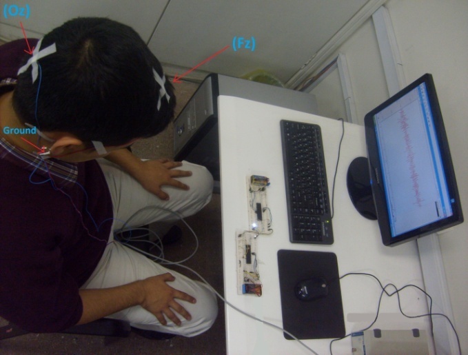 | Figure 1. Electrode positioning and the twinkling light sources used in this study. The monitor and the surrounding light sources are turned off during data recording periods |
Five different horizontal distances (D) of 4, 14, 24, 44 and 64 cm were examined between the two sources, as the plane of the sources were located 60 cm away from the subject as shown in Figure 2. Therefore, the inter-sources distances of D=4, 14, 24, 44 and 64 cm are equivalent to a horizontal angle of 3.8°, 13.4°, 22.6°, 40.2° and 56° respectively. Considering a constant distance of 60 cm between the subject and the light sources plane during all experiments, for simplicity from now on the inter-sources distances are only represented by their distance in centimetre instead of the angles between them in degree. Wider inter-sources distances than 64 cm are not applicable since one of the sources falls out of the visual field when looking at the other one. These stepwise distances were selected arbitrary to cover the complete field of view from D=4 cm to D=64 cm. As the results show (see Fig 6), selection of other steps for inter-sources distances would provide comparable results.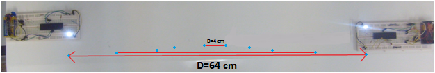 | Figure 2. Different inter-sources distances considered in this study |
A luminance meter was located in place of the subject's eye for a more accurate measurement of the experimental parameters. The background luminance of the experiment was around 40 to 140 cd/m2 for various subjects and at different times while the source luminance was around 11000 to 13000 cd/m2. Therefore, the modulation depth[20] varied between 97.5 to 99.2% at different inter-sources distances, which can be assumed almost constant in all cases.
2.2. Data Acquisition and Analysis
SSVEP signals were recorded for eight subjects (males, age between 25±2 years) all with normal eyesight in the Biomedical Engineering Laboratory of the . Each subject was asked to look at the light sources for a period of 60 seconds, one at a time, while the other source was also active at the predefined distances from the main light source. In the meantime, the SSVEP signals were recorded. This procedure was repeated twice for each light source producing 2 minutes of SSVEP signal for each of the light sources and 4 minutes of data for the two light sources for each subject and each inter-sources distance. This procedure was repeated for all five inter-sources distances of 4, 14, 24, 44 and 64 cm. As a first stage, a Band pass filter of 5-45 Hz was applied to all signals in the dataset. Next, due to real-time applications of BCI systems, each of the 4 minutes long recorded SSVEP signals for each source and for each inter-sources distance is divided into short non-overlapping segments each of durations of 0.5, 1, 2 and 3 seconds sweeps producing 480 segments each of length of 0.5 seconds, 240 segments each of length of 1 seconds, 120 segments each of length of 2 seconds, and 80 segments each of length of 3 seconds. Our studies showed that for SSVEP sweeps less than 0.5-second length, the accuracy of the classifiers were reduced significantly, therefore, the shortest segment length were limited to 0.5 second. For a more accurate study on this subject, the outlier segments (the segments with Signal to Noise Ratios (SNR) less than 1) are determined and excluded from the data set. The SNR of the signal is defined as follows[21]: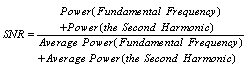 | (2) |
where the sum of the powers of the fundamental frequency and its second harmonic is divided by the average power. The average power is calculated by summing the power of the signal in a window of width of three times of the frequency resolution of the signal around both the fundamental frequency and its second harmonic. The frequency resolution of each signal is defined as the inverse of the sweep duration. For each of the remaining segments a temporal domain feature vector is defined and used in the next step as follows. First, forward-backward Autoregressive (AR) model (see Equation (3))[22] of orders from 1 to 15 is developed and the resulting coefficients are used as signal features. Due to the limited number of signal segments used for training of the AR models, the upper limit of the models are bounded to a maximum value of 15 in this study. | (3) |
In Eq. (3)  s are the AR coefficients, is the model order and
  is an additive white noise with a zero mean and finite variance[22].Therefore, for each sweep of length 0.5 seconds the total data matrix will be of dimension 480×1 to 480×15, (480 observations and 1 to 15 AR features). For other sweeps, this will be of sizes 240×1 to 240×15, 120×1 to 120×15 and 80×1 to 80×15.As the next step, the three different classification techniques of the Linear Discriminant Analysis (LDA), the Support Vector Machine (SVM) and the Naïve Bayes are considered to classify each segment as if the first or the second light source is in the centre of attention of the subject. For training of all classifiers in classification step, the data set is shuffled and divided into the training and test sets of sizes of 80% and 20%, respectively. The process is repeated 50 times and the accuracy results were averaged for each subject separately over the test sets.In addition, the ITR for the above mentioned three classifiers for all sweeps of 0.5, 1, 2, and 3 seconds is calculated and compared.
3. Results
In this section, the results of the application of the proposed method to the signals in the dataset are presented. First, the average SNR of the segments are calculated using equation (2) over all of the eight subjects and over all available segments. The results are shown in tables 1 and 2 for sources of frequencies of 15 Hz and 20 Hz respectively. Due to the large value of SNR in all cases, it is not necessary to apply any pre-processing method to the dataset. It worth to note that the SNR values for the sources with twinkling frequency of 15 Hz are almost always greater than of those for 20 Hz.| Table 1. Mean SNR values over all available segments while subjects are looking at 15 Hz twinkling light source |
| | Mean | D=4 cm | D=14 cm | D=24 cm | D=44 cm | D=64 cm | | sweep =0.5 s | 2.4670 | 1.9972 | 2.3532 | 2.5330 | 2.4971 | | sweep = 1 s | 2.3372 | 2.3480 | 2.5340 | 2.9800 | 2.5145 | | sweep = 2 s | 3.0750 | 2.9976 | 3.4417 | 3.6524 | 3.3074 | | sweep = 3 s | 5.1152 | 4.8138 | 5.2958 | 5.2501 | 5.2149 |
|
|
| Table 2. Mean SNR values over all available segments while subjects are looking at 20 Hz twinkling light source |
| | Mean | D=4 cm | D=14 cm | D=24 cm | D=44 cm | D=64 cm | | sweep =0.5 s | 1.9687 | 1.9543 | 2.0830 | 2.1006 | 2.0955 | | sweep = 1 s | 1.8139 | 1.8351 | 1.8899 | 1.9900 | 1.9377 | | sweep = 2 s | 2.9273 | 3.2996 | 4.1635 | 3.7171 | 4.0944 | | sweep = 3 s | 2.8383 | 3.0929 | 3.2458 | 3.1779 | 2.7383 |
|
|
To evaluate the performance of the LDA, the SVM and the Naïve Bayes classifiers, the mean and standard deviation (STD) values for the accuracy of the data in the test sets over the AR model orders and for 5 different inter-sources distances are computed and shown in Figures 3, 4 and 5, respectively.As it can be seen in Figure 3, although for all cases the performance of the LDA classifier is reduced by decreasing the inter-sources distances from D=64 to D=4 cm (with a p-value of p<0.001), however its performance for D=24, 44 and 64 cm are almost similar for 0.5s and 3s sweeps (0.05<p<0.5), while for 1s and 2s sweeps, D=64 cm is almost always better than the other cases (p<0.001).It should be noted that by increasing the sweep lengths, the Mean accuracies of the LDA classifier generally increases over all subjects. It can be concluded that the best AR orders for all sweeps and for all distances is 12-14.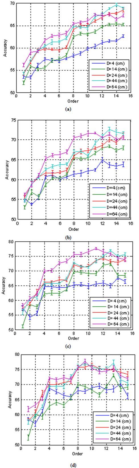 | Figure 3. Mean and STD values for sweeps of length (a) 0.5s (b) 1s (c) 2s (d) 3s over all subjects for different AR orders and various inter-sources distances (D) with the LDA classifier |
As shown in Figure 4, for all sweeps the performance of the classifier for D=24, 44 and 64 cm are almost similar (0.05<p<0.5) and its performance for D=4 cm is the worst (p<0.001). With the SVM classifier, the best AR models are from 12 to 14 and as the LDA case, by increasing the sweep lengths the mean accuracy over the subjects also increases.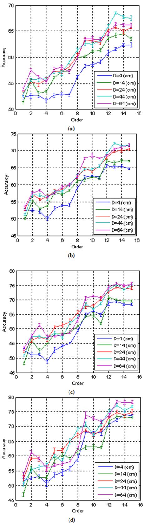 | Figure 4. Mean and STD values for sweeps of length (a) 0.5s (b) 1s (c) 2s (d) 3s over all subjects for different AR orders and various inter-sources distances (D) with the SVM classifier |
As it can be seen in Figure 5, by inter-sources distance decrements, the performance of the Naïve Bayes classifier decreases (p<0.001), however the performance of the classifier for D=64 cm and D=44 cm are almost similar (0.05<p<0.5). The best AR orders are 9, 12-14. 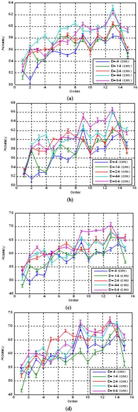 | Figure 5. Mean and STD values for sweeps of length (a) 0.5s (b) 1s (c) 2s (d) 3s over all subjects for different AR orders and various inter-sources distances (D) with the Naïve Bayes classifier |
As it was previously stated, the best AR orders of the LDA, the SVM and the Naïve Bayes classifiers within all sweeps and distances were 12-14. In order to compare different classifiers, the AR model of order 13 was chosen due to its generally better performance. Figure 6 illustrates the accuracies of all three classifiers for the AR order of 13 over different inter-sources distances. As it can be seen, the performance of the Naïve Bayes classifier is worse than others, while the performance of the LDA and the SVM are similar for all sweeps. Generally, as inter-sources distances increase, accuracy of all three classifiers also increases, however the performance of all classifiers for D=64 cm are less than those for D=44 cm, occasionally. As it was mentioned before, by increasing the length of the sweeps, the performance of all classifiers also increases over all inter-sources distances.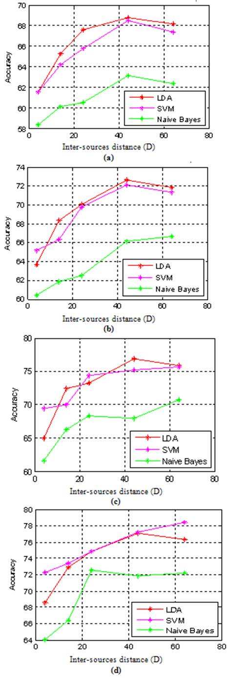 | Figure 6. Accuracy of the classifiers over inter-sources distances (D) for (a) 0.5s (b) 1s (c) 2s (d) 3s of 13’ order |
Figure 7 illustrate ITRs of three classifiers for all sweeps over different inter-sources distances (D) for 13th AR order. It should be noted that all ITR values are calculated using equation 1 for N (the number of classes) equals to two corresponding to 2 external light sources. As it can be seen for all three classifiers, the ITR for sweep length of 0.5s is always better than other cases. ITRs of the LDA and the SVM classifiers are close to each other, while they outperform the Naïve Bayes classifier. In addition, the turning point of inter-sources distances is D=44 cm.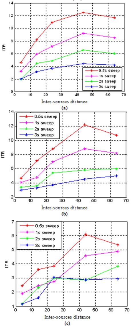 | Figure 7. Information Transfer Rates (ITRs) in (a) the LDA (b) the SVM (c) the Naïve Bayes classifier for all sweeps |
4. Discussion
In this research, we have concentrated on the effect of inter-sources distances (D) on the accuracy of the SSVEP -based BCI systems. In particular the inter-sources distances of D=4, 14, 24, 44 and 64 cm were studied. In addition, due to the usage of AR models for feature definition for the SSVEP signals, selection of best AR model was also considered in this study. More over three different classifiers of the LDA, the SVM and the Naïve Bayes were examined.According to the results shown in figures 3 to 5, in all classifiers, the mean accuracy over the subjects increases by the increment of the sweep lengths. A reason for this could be the more accurate AR model parameters estimated from longer signals. In addition, the overall performances of the classifiers are also improved by increasing the AR model orders. This is more obvious for the AR orders up to 13 and 14 and especially using the shorter sweep lengths. Moreover, it can be seen that the AR models of order 13 could better models the SSVEP signal producing the highest accuracy in general. According to figures 3 to 5, it can be concluded that by increasing the inter-sources distances from D=4 cm to D=64 cm, the accuracy of the BCI system is generally increasing. That is due to less interference of each flickering LED with the other one in higher inter-sources distances. According to Fig 6 which displays the accuracy of the AR model with order 13 exclusively, it worth to note that the inter-sources distance of D=44 cm is the turning point of the accuracy curves in general. This is because D=64 cm is more distant to the eyes than D=44 cm which could probably affect the luminance entering the visual field. For practical applications, using the inter-sources distance of D=24 cm is more desirable due to the shorter inter-sources distance despite of its lower accuracy. This is because using shorter inter-sources distance could help to reduce the overall system size in such BCI applications as the electronic telephone where 12 light sources are used. Moreover, the performance of the LDA and the SVM classifiers, which are almost similar, outperform the Naïve Bayes one. Figure 7 shows the ITRs for five inter-sources distances of D=4, 14, 24, 44 and 64 cm, four sweeps of 0.5, 1, 2 and 3 seconds, three different classifiers of the LDA, the SVM and the Naïve Bayes for the best AR order of 13. As it can be seen, for all classifiers the 0.5s sweep has higher ITR values with the Naïve-Bayes classifier showing the worst performance.It must be mentioned that no similar study has been done on the effect of the inter-sources distances on the performance of the SSVEP based BCI systems in the past. To the knowledge of the authors, the only comment regarding the effect of the inter-sources distance is given in [13] where it was qualitatively concluded that for closer distances the general SSVEP signal shows smaller amplitude in the time domain.
5. Conclusions
In this paper, the effect of the inter-sources distances on the accuracy of the SSVEP-based BCI systems was investigated. It was showed that an inter-sources distance of D=44 cm (equivalent to the visual angle of 40.2°) could produce the highest accuracy among the other inter-sources distances that were studied. For a more practical BCI system, however, the inter-sources distance of D=24 cm (equivalent to the visual angle of 22.6°) is proposed due to a relatively shorter inter-sources distance with an acceptable accuracy rate.Using the AR coefficients as signal features and either the LDA or the SVM classifiers, it was also showed that an AR model of 13 outperforms other possible AR model orders that were studied.Finally, it was showed that a signal length of 0.5 second could provide a more practical online information transfer rate.
References
| [1] | K. Revett (2007) On the Use of Rough Sets for Artifact Extraction from EEG Datasets. IEEE, Frontiers in the Convergence of Bioscience and Information Technologies 425–430. doi: 10.1109/FBIT.2007.144 |
| [2] | B. Hamadicharef, S. M. Xu Aditya (2010) Brain-Computer Interface (BCI) based Musical Composition. IEEE, International Conference on Cyberworlds, 282-286. doi: 10.1109/CW.2010.32 |
| [3] | J. V. Odom, M. Bach, M. Brigell et al (2009) ISCEV standard for clinical visual evoked potentials. Springer-Verlag , Doc Ophthalmol. doi 10.1007/s10633-009-9195-4 |
| [4] | B. Link, S. Ruhl, A. Peters, A. Junemann, F. K. Horn (2006) Pattern reversal ERG and VEP – comparison of stimulation by LED, monitor and a Maxwellian-view system. Springer, Documenta Ophthalmologica, 112: 1-11. doi: 10.1007/ s10633-005-5865-z |
| [5] | H. Shen, L. Zhao, Y. Bian, L. Xiao (2009) Research on SSVEP-Based Controlling System of Multi-DoF Manipulator. , 171–177. |
| [6] | E. C. Lalor, S. P. Kelly, C. Finucane et al (2005) Steady-State VEP-based brain-computer interface control in an immersive 3D gaming environment. EURASIP, Journal on Applied Signal Processing 19: 3156–3164. |
| [7] | G. R. Muller-Putz, R. Scherer, Ch. Brauneis, G. Pfurtscheller (2005) Steady-state visual evoked potential (SSVEP)-based communication: impact of harmonic frequency components. Institute of physics publishing, Journal of neural engineering 2:123–130. |
| [8] | T. M. Srihari Mukesh, V. Jaganathan, M. R. Reddy (2006) A novel multiple frequency stimulation method for steady state VEP based brain computer interfaces. IOPscience, Physiological Measurement 27:61–71. |
| [9] | Po-Lei Lee, Jyun-Jie Sie, Yu-Ju Liu, Chi-Hsun Wu (2010) An SSVEP-Actuated Brain Computer Interface Using Phase-Tagged Flickering Sequences: A Cursor System. Annals of Biomedical Engineering 38:2383–2397. |
| [10] | M. Middendorf, G. McMillan, G. Calhoun, and K. S. Jones (2000) Brain-computer interfaces based on the steady-state visual-evoked response. IEEE Transactions on Rehabilitation Engineering 8(2): 211–214. |
| [11] | P.-L. Lee, C.-H. Wu, J.-C. Hsieh, Y.-T. Wu (2005) Visual evoked potential actuated brain computer interface: a brain-actuated cursor. Electronics Letters 41:832-834. doi: 10.1049/el:20050892 |
| [12] | B. S. Reddy, O. A. Basir, S. J. Leat (2007) Estimation of driver attention using Visually Evoked Potentials. IEEE, Intelligent Vehicles Symposium 588-593. doi: 10.1109/IVS.2007.4290179 |
| [13] | S. Fuchs, S. K. Andersen, Th. Gruber, M. M. Müller (2008) Attentional bias of competitive interactions in neuronal networks of early visual processing in the human brain. ELSEVIER, NeuroImage, 41:1086-1101 |
| [14] | D. J. McFarland, W. A. Sarnacki, J. R. Wolpaw (2003) Brain-computer interface (BCI) operation: optimizing information transfer rates. Elsevier, Biological Psychology 63:237-251 |
| [15] | S. N. Resalat, S. K. Setarehdan, F. Afdideh, A Heidarnejad (2011) Appropriate Twinkling Frequency and Inter-source Distances Selection in SSVEP-based HCI Systems. To be published, , icsipa2011. |
| [16] | F. Faradji, R. K. Ward, G. E. Birch (2011) Toward development of a two-state brain–computer interface based on mental tasks. IOP PUBLISHING, JOURNAL OF NEURAL ENGINEERING, 8, 046014, doi:10.1088/ 1741- 2560/ 8/4/ 046014 |
| [17] | M. Huang, P. Wu, Y. Liu, L. Bi, H. Chen (2008) Application and Contrast in Brain-Computer Interface between Hilbert-Huang Transform and Wavelet Transform. IEEE, the 9’Th International Conference for Young Computer Scientists, 1706-1710. |
| [18] | Po-Lei Lee, Jen-Chuen Hsieh, Chi-Hsun Wu, Kuo-Kai Shyu (2008) Brain computer interface using flash onset and offset visual evoked potentials. Elsevier, Clinical Neurophysiology, 119: 605–616. |
| [19] | Zhenghua Wu (2009) The Difference of SSVEP Resulted by Different Pulse Duty-cycle. IEEE, International Conference on Communications, Circuits and Systems 605-607 |
| [20] | D. Z. Molina, G.G. Mihajlovic, V. Aarts (2010) Phase synchrony analysis for SSVEP-based BCIs. IEEE, 2’nd International Conference on Computer Engineering and Technology (ICCET) 2:329-333. doi: 10.1109/ICCET.2010.5485465 |
| [21] | Z. Wu, Y. Lai, Y. Xia, D. Wu, D. . (2008) Stimulator selection in SSVEP-based BCI. Elsevier, Medical Engineering and Physics 30:1079–1088 |
| [22] | V. Jandhyala, , R. Mittra (1994) FDTD signal extrapolation using the forward-backward autoregressive (AR) model. IEEE, Microwave and Guided Wave Letters 4:163-165 |
| [23] | M. Dondrup, A. T. Hüser, D. Mertens, A. Goesmann (2009) An evaluation framework for statistical tests on microarray data. Elsevier, Journal of Biotechnology, 140:18-26. |
 Abstract
 Reference
 Full-Text PDF
 Full-Text HTML