1. Introduction

Traveling waves transmit information through space and always an excitable medium serves to promote propagation. an excitable medium is typically comprised of a continuous set of locally excitable regions,which can be both independently stimulated and inhibited.these media exhibit a sensitivity threshold blow which the media persist undisturbed at a stable resting state.while subthreshold perturbations are rapidly diminished, greater than threshold signals induce an abrupt local transformation within a portion of the medium. shortly after this change occurs, the region becomes transiently refractory to further perturbation, after which it relaxes to the resting state.

The bioelectric activity of cardiac cells results from the transport processes of ionic species across the membrane through voltage-gated ion channels. The ion channels act as gates that regulate the permeabilities of sodium, potassium and calcium ions. At rest, the cell maintains a constant, negative transmembrane voltage, called the resting potential. However, if a strong enough depolarizing current is passed through the membrane, the cell departs from equilibrium and responds with a sharp change in the transmembrane voltage followed by a return to the resting state. This rapid course of the transmembrane voltage is called action potential (AP) that is the fastest form of communications in the cardiac excitable tissue. Conduction of AP in the heartoccurs by electrotonic mechanisms, in which the local release of stored energy is spent to trigger similar cellular events in adjacent regions. Action potential waves are self-sustaining signals in the sense that they retain their amplitude and shape at the expense of energy provided by the cell metabolism. During normal sinus rhythm, AP waves are periodically initiated by the pace maker cells of the sinoatrial node and propagate through atria and ventricles. Cardiac arrhythmias are disorders of either wave initiation or wave propagation.

Modeling studies have a long-standing tradition and play very significant role in cardiac electrophysiological research. Mathematical models and computer simulations play an increasingly important role in cardiac arrhythmia research. Electrophysiological models have complete description from details of cardiac cells processes and can be used for accurate study in cellular level. One of the most important applications of these theoretical studies is the simulation of the human heart, which is important for a number of reasons. First, the possibilities for doing experimental and clinical studies are very limited. Second, animal hearts used for experimental studies may differ significantly from human hearts [heart size, heart rate, action potential (AP) shape, duration, and restitution, vulnerability to arrhythmias, etc]. Finally, cardiac arrhythmias, especially those occurring in the ventricles, are three-dimensional phenomena whereas experimental observations are still largely constrained to surface recordings[1]. Computer simulations of arrhythmias in the human heart can overcome some of these problems.

The excitable behavior of cardiac tissue has traditionally been described using either cellular automata (CA) models or partial differential equation (PDE) models. The first models used to study re-entry by Wiener & Rosenblueth (1946)[2] and fibrillation by Moe (1964)[3] were CA models. In these models, cells have a discrete state (resting, excited, refractory), and rules describe state transitions depending on the current state of the cell and its neighbors. Because of their computational simplicity, CA models have been used extensively in whole heart models to reproduce normal and abnormal excitation sequences. However, in order to precisely model properties such as action potential duration and conduction velocity restitution and wave front curvature effects, large numbers of different states and a set of complex transition rules is needed. This will lead to the loss of computational simplicity of the CA model. Therefore, for studying the mechanisms behind onset and dynamics of reentrant arrhythmias, for which properties such as curvature and restitution are essential, usually PDE models are used.

Among the PDE based models phenomenological models such as FitzHugh–Nagumo like models (FitzHugh 1960, 1961[4,5], Nagumo 1962[6], Aliev and Panfilov 1996[7]) and the Fenton–Karma model (Fenton and Karma 1998[8]) are computationally very efficient, but lack lectrophysiological detail. The first generation of cardiac cell models aimed to reproduce the action potential based on available experimental information about the voltage and time dependence of ion channel conductance data, reviewed in Rudy (2006)[9]. The ion channel kinetics are based on those used in the Hodgkin–Huxley model of the squid giant axon (Hodgkin and Huxley 1952[10]), first adapted for cardiac Purkinje cells by Noble (Noble 1962[11]). The Beeler Reuter model (Beeler and Reuter 1977[12]) was the first ionic model of ventricular myocytes, as distinct from models of Purkinje cells.

Second-generation models are more computationally intensive to solve than first-generation models because they include more state variables for ion channels, pumps and exchangers, as well as the intracellular ion concentrations and transfer. The first second-generation model was the DiFrancesco-Noble model of Purkinje cells (DiFrancesco and Noble 1985[13]), and other early second-generation models of ventricular cells include the Luo Rudy dynamic (LRd) model (Luo and Rudy 1994[14]) and the Noble 1998[15] model for guinea pig ventricular cells. Both first and second generation ionic models contain a lot of electrophysiological detail, but are computationally very expensive. We therefore need a model of an intermediate type. Bernus[16] in 2002 constructed a relatively simple ionic model for human ventricular cells based on the second generation Priebe–Beuckelmann ionic model (Priebe and Beuckelmann 1998[17]). The disadvantage of this intermediate type model is that the Priebe–Beuckelmann model itself is based on only a limited amount of at that time available human cardiac cell data.

To be able to study human whole heart activities and how these are linked to (sub) cellular processes such as ion channel mutations, a human cardiac cell model that is both detailed and computationally efficient is needed. So in this computational study we use an efficient PDE model (Ten Tusscher&Panfilov 2006)[18] with two mentioned characteristics. This model is based on partial differential equation method. In the second section of this article we explain the equation of action potential propagation, numerical method for solving this equation and characteristics of represented excitable media, respectively. Then the stimulation ways that we apply for generating AP in the excitable medium are described and at end of this section our proposed wave propagation algorithm is represented. In third section firstly single action potential in the ventricular cardiac cell is simulated and in continue, our simulations contain action potential propagation in one-dimensional(1D) and two-dimensional(2D) states. All simulations were written in DELPHI.

2. Methods

2.1. Numerical Method

Action potential generation and propagation in a one- dimensional strand of ventricular muscle and in a two- dimensional grid of cardiac ventricular cells was described using the following differential equation as in[19]:

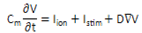(1)

Where V is the transmembrane potential,C_m is the transmembrane capacitance, D is the diffusion coefficient, I_ion are currents constituted by various ions across the cell membrane and I_stim is the external current signal.

For numerical solving of two-dimensional wave propagation, central finite difference method is used with a time step of 0.02 millisecond and a space step of 0.25 millimeter.This method can be derived from performing Taylor expansion of V at x as follows:

(2)

(3)

By considering h≪1 and adding the equations (2) and (3) central finite difference approximation is achieved as equations (4) :

(4)

We assume C=1μF/cm² and for D we use D = 0.00154 cm²/ms in one dimensional and two dimensional grid of cells simulations to obtain a maximum planar conduction velocity (CV) of 68 cm/s consistent with measurements in human ventricular tissue[18], and a value of D = 0 cm²/ms for single cells.

2.2. Excitable Media

In this work, for studying the 1D wave propagation we assume that cardiac cells are connect to one another, forming an excitable cellular cable including 50 cells at the same direction and then for 2D wave propagation study the simulations are performed on a square excitable medium with 80 cells in both x and y directions.

2.3. Stimulation Methods

It's mentioned that for generating the propagating waves in an excitable medium stimulation signals are always required. In this simulation study, at first in 1D propagation state, by applying the stimulation at one side of our excitable cable the AP wave propagates along the cable. In 2D propagation state, we apply the stimulation in two different ways. Firstly by stimulating the bottom side of represented square excitable medium and secondly by an external stimulus, applied at the left down corner of excitable medium.

2.4. Wave Propagation Algorithm

In this article we represent a computational algorithm for action potential propagation as given in flowchart(1).This flowchart shows the procedure of 2D action potential propagation. According to flowchart(1), x and y are two spatial variables and t is time variable, applied in our proposed algorithm. Moreover X_end , Y_end and t_end are final values, assigned to two spatial parameters and time parameter respectively. Likewise ΔX and ΔY indicate two space steps and Δt indicates time step of algorithm. The procedure of 1D action potential propagation is also similar to 2D one, but instead of two spatial variables and consequently two space loops in the algorithm, there is only one spatial variable and naturally one space loop.

In each loop and in each stage, computations continue until the certain variable of each loop doesn't become more than its assigned final value. If it becomes more than the mentioned final value, the space loops by adding the space step to spatial variable and the time loop by adding the time step to time variable enter to next computational stage. In final stage the computations will be finished and the desired output as AP signal will be achieved.

3. Results

3.1. Action Potential of Single Cell

The typical cardiac action potential has 5 phases from 0 up to 4 including: (0) depolarization or upstroke phase,(1) partial repolarization or notch phase (2) plateau phase (3) repolarization phase and (4) resting membrane potential phase[20]. In this section at first AP response of single cell is simulated. Figure(1) illustrates the simulation of AP in cardiac ventricular myocardium cell. According to this figure, five phases of action potential signal is observable. In figure(1) vertical axis depicts the transmembrane voltage in millivolt and horizontal axis shows time in millisecond.

3.2. One-dimensional (1D) Action Potential Propagation

In this stage we study the AP generation and its propagation in 1D state.Figure(2) demonstrates this type of propagation.Vertical axis in this figure represents the transmembrane voltage and horizontal axis shows the number of cells that formes 1D excitable cable. Figure(2) clearly illustrates when we stimulate the start of the excitable cable, AP wave initiates and propagates along the horizontal axis.

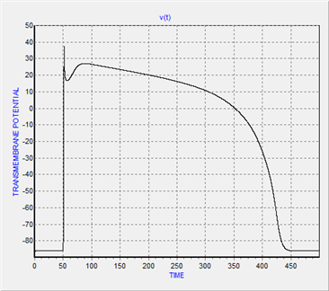Figure 1. Action potential of single cardiac cell(ventricle myocardial cell)

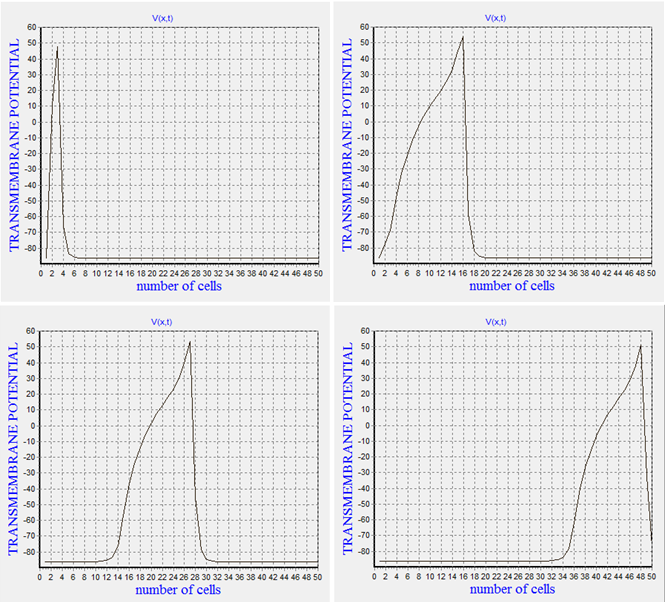Figure 2. The procedure of action potential propagation in one-dimensional(1D) state

According as we observe in figure(2) AP wave naturally continues in every point of excitable cable in a specific duration and the repolarization process starts from region that depolarization process was initiated and then at the same direction that depolarization wave has proceeded, repolarization process will be continued too. According to all or nothing principle that is true in all natural excitable media, when an AP occurs in any point of excitable medium the depolarization process travel through space.This law is also confirmed in our represented excitable medium.

3.3. Two-dimensional (2D) Action Potential Propagation

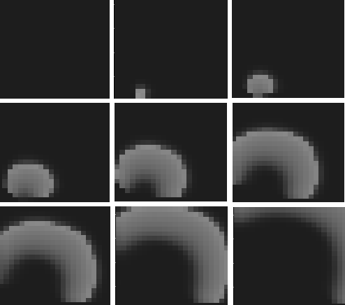
In this stage, we survey the 2D action potential propagation according to our represented algorithm and 2D excitable medium and also based on the proposed efficient model .The propagation quality of two different wave fronts as plane wave front and as convex wave front will be studied. One of the most important characteristics of 2D propagation is curvature. A plane wave front conserves its length locally and thus each depolarized cell needs to depolarise only one cell in front of it. In contrast the length of a convex wave front steadily increases, and therefore the current initiating depolarisation spreads to a larger area than that for a plane front. As a result, convex fronts propagate more slowly than a plane front[21]. Now for validating of our represented propagation algorithm and excitable medium we study this scientific reality in this section.

Figure(3) illustrates the procedure of action potential propagation in 2D excitable medium as a plane wave front. In the beginning, we don't apply any stimulation and the excitable medium is in the resting state. By applying the stimulation to the entire bottom side of the medium, excited status is formed in the cells and depolarization signal as a planar wave front starts to propagate in the tissue until it's gently damped and the excitable medium regains its own resting state. Similar to 1D state all or nothing principle is confirmed in the represented 2D excitable medium.

Figure 3. 2D action potential propagation as a plane wave front (series of snapshots 0,3,6,8,10,12 milliseconds after start of propagation, from top row to bottom row respectively and in each row from left side to right side)

In the second time according to figure(4), a point stimulation is applied to the medium. Like the previous case,in the absence of any stimulation the medium remains as is. When we apply an external stimulus at the left down corner of excitable medium, a convex wave front is formed that after damping, excitable medium returns again to rest.In both figure(3) and figure(4),dark color and light color depict resting state and excited status of excitable medium, respectively.

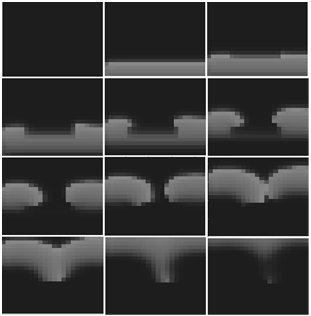
Figure 4. 2D action potential propagation as a convex wave front (series of snapshots 0,0.5,2,4,6,8,10,12,14 milliseconds after start of propagation, from top row to bottom row respectively and in each row from left side to right side)

According to the recorded times of snapshots in figures(3) and (4), it's clearly observable that convex wave front needs more time than plane wave front to traverse the medium. On the other hand the plane wave propagation speed is more than convex wave front. Now for more validating of our work, we study the effect of obstacles on the AP propagation in our represented excitable medium.

In the normal heart, rhythmic cardiac contraction is coordinated through non-linear electrical waves of excitation that smoothly propagate through the cardiac tissue. A common cause of cardiac arrhythmias are reentrant waves. The term reentry was coined to describe a wave front that reenters and hence re-excites the same tissue again and again as opposed to the normal planar wave front emitted by the sinus node that excites all tissue only once.

In two dimension tissue, reentry can be caused by a wave front curved around an inexcitable obstacle that This so- called anatomical re-entry (Wiener & Rosenblueth 1946[2]; Winfree 1980[22]; Zykov 1987[23]). in fact the dead regions of the cardiac tissue play the role of inexcitable obstacles.An AP wave front, for successfully expanding in tissue, requires that there be a sufficient number of Na ions that can diffuse into adjacent resting cells and raise the membrane potential to the firing threshold. Hence, in this study we creat the local inexcitable obstacle as a dead tissue with considering the sodium ion conductance equal to zero in the excitable medium.

Figure 5. Effect of inexcitable obstacle as a dead tissue on the normal action potential propagation

As given in figure(5), a rectangular obstacle in the medium is considered with conditions that we mentioned before. According to this figure its observed the considered obstacle that exists in the passing way of wave front disorders it. This perturbation causes changes in normal AP propagation in the grid, which disturbs the normal cardiac rhythmic pattern and arrhythmia condition is achieved. The cumulative effect of the disturbance in the abnormal cardiac rhythmic pattern forms a reentry in the location where obstacle exists. The reentry is formed because the dead region of the tissue acts as an obstacle for normal AP propagation. As time elapses the reentry waves move to all regions of grid and thus causing total arrhythmic pattern in the grid.

4. Discussion

It's mentioned that the cardiac electrical activity is known as action potential (AP) that travels through atria and ventricles in a synchronized fashion. In this article a human cardiac cell model that is both detailed and computationally efficient was used.

Confirmation of all or nothing principle in the represented excitable media was an evidence for validity of our both computational algorithm and excitable mediums. According to this principle in the excitable media an AP signal either occurs fully or doesn't occur at all. In continue for more validation of our work, we compare the quality of AP propagation as plane wave front and convex wave front. In this issue we illustrated that the speed of a plane wave front is more than convex one. For final validation of our work we investigated the effect of inexcitable obstacles on AP propagation. For this purpose we refered to this concept that a wave front, for successfully expanding in tissue, requires recruiting an adequate supply of sodium ions(Na) that can diffuse down a concentration and voltage gradient into adjacent resting cells thereby depolarizing the local membrane potential to the Na channel opening threshold. Because recently recruited Na channels inactivate, they must be rapidly replaced with newly recruited channels in order to prevent wave front collapse. the process of charge diffusion and subsequent opening of resting Na channels adjacent to the wave front is referred as a recruiting process. So we created our desired inexcitable obstacle by considering Na ion conductance (G_Na) equal to zero in a specific area of medium and it was observed the reentry was formed in this manner that is one of main reasons leading to the cardiac arrhythmias.

There are two main limitations to the PDE model we proposed in this paper. First, because of the absence of sodium and potassium dynamics in this model, we cannot investigate the development of conditions such as ischaemia and hyperkalaemia. Second, because of the absence of intracellular calcium dynamics in this PDE model it cannot be used for studying conditions such as calcium overload, spontaneous calcium release, calcium-induced alternans and the influence of calcium dynamics on wave break. Furthermore because of using personal computer in this computational study, we had some restrictions for implementation of 2D simulations in larger scales.

5. Conclusions

In this work, we represented an algorithm and subsequently the excitable media for studying the AP formation and its propagation in 1D and 2D states. The simulations were implemented using an efficient PDE model. Results approved that proposed efficient model, represented algorithm and excitable media are suitable for simulation of AP propagation in cardiac tissue.

Because of capability of represented computational algorithm, it can be extended to 3D state for simulation of three-dimensional AP propagation in cardiac tissue. Moreover since ionic concentrations like sodium and calcium have a significant effect on formation and controlling the cardiac arrhythmias, the offered algorithm, excitable media and proposed PDE model are useful for investigating these issues. In addition, the presented algorithm can be used for simulation of AP propagation in any electrophysiological models.