1. Introduction

Breast cancer is the most common cancer and the second leading cause of cancer death in women in Western countries. Imaging has a crucial role in the workup of patients with breast cancer with contributions to early detection through screening, diagnosis and associated image-guided biopsy, treatment planning, and treatment response monitoring [2].

Dynamic contrast-enhanced magnetic resonance (MR) imaging is the most sensitive radiological method for detecting breast cancer [3]. Although, X-Ray mammography has shown considerable success in screening for the early detection of breast cancer, some limitation exist, such as low specificity leading to unnecessary biopsies, presentation of cancer lesions as radio graphically occult in dense breasts, and the inherent limitations of two-dimensional (2D) projection image data. Thus, extensive efforts in recent years have included the use of magnetic resonance imaging (MRI) and sonography as complementary imaging modalities to improve breast-interpretation [2]. Currently, breast MRI has a high sensitivity for breast cancer detection reported as high as 94-100%, but a lower specificity, reported as 37-97%[4].

In the clinical reports, the Artificial Neural Network (ANN) has been widely applied in breast cancer diagnosis using different features [5-7]. By presenting examples of known class specification, the neural network is able to learn the distribution patterns of “typical” features of each class (supervised learning). Afterwards, the network can be used to separate non-determined data into the different classes and to calculate the probability for belonging to each of the classes [8].

In this study, a forward selection method is applied to find the best features to the classification of breast cancer. Also, some classifiers are used to classify breast cancer into two groups; benign and malignant lesions.

This paper is organized as follows. The database and its quantitative parameters are described in II. Feature selection method and applied classifiers is explained in section III. In section IV, simulation results are summarized on tables to show the performance and the comparison of applied methods. Discussion on the topic is in section V. Finally, the paper is concluded in section VI.

2. Material

2.1. Database

The database analysed in this study included a total of 112 histology-proven lesions, 86 malignant (41 mass, 45 non-mass) and 26 benign (17 mass, 9 non-mass). These cases were collected from 2004 to 2006. Patients with suspicious findings or with biopsy-proven cancer were invited to participate in a breast MRI research study. Only cases with a clearly visible lesion in a clean background were selected. Cases with multiple poorly differentiable lesions, locally advanced diseases receiving neoadjuvant chemotherapy, or with severe motion artifact, were excluded. The age of patients with malignant cancer ranged from 31 to 80 years (53±11, median 50), and the patients with benign diseases were younger, range 30-74 years old (49±11, median 47). Mass-type lesions were determined based on the clear boundaries and strong enhancements. Lesions presenting as non-mass-like enhancement (or lesions without mass effect) were identified as those presenting diffuse enhancement with ill-defined tumor margins. An experienced radiologist evaluated each lesion and determined whether it should be designated a mass or a non-mass. Table 1 summarizes the histological types of these four groups of lesions. This database was approved in the University of California, Irvine by the institutional review board and in compliance with Health Insurance Portability and Accountability Act (HIPAA) regulations. Written informed consent was obtained from all subjects [9].

Table 1. Histological Types of Lesions in the Four Groups: Malignant Mass, Benign Mass, Malignant Non-mass and Benign Non-mass Tumor group Number Percentage Malignant mass 43 37 IDC (invasive ductal carcinoma) 27 23 DCIS (ductal carcinoma in situ) 4 3.5 ILC (invasive lobular carcinoma) 8 7 Mixed 4 3.5 Benign mass 19 16 Fibroadenoma 15 13 Mixed 4 3 Malignant non-mass 45 39 IDC (invasive ductal carcinoma) 9 8 DCIS (ductal carcinoma in situ) 12 10 ILC (invasive lobular carcinoma) 16 14 Mixed 8 7 Benign non-mass 9 8 Fibrocystic changes 8 7 Mixed 1 1

2.2. Quantitative Analysis of Lesion Shape Features and Enhancement Texture

2.2.1. Shape Features

Eight features were used to describe the shape of a lesion: volume, surface area, compactness, NRL (normalized radial length) mean, sphericity, NRL entropy, NRL ratio and roughness. Compactness is defined as the ratio of the square of the surface area to the volume of the lesion—with a sphere having the lowest compactness index and an irregular undulating shape, such as a spiculated lesion, having a higher compactness index. The features based on the normalized radial length (NRL) describe contours and the finer shape of the lesion. NRL is defined as the Euclidean distance from the object’s centre (centre of mass) to each of its contour pixels and normalized relative to the maximum radial length of the lesion[9, 10].

2.2.2. Texture Features

Radio graphically, texture is defined as a repeating pattern of local variations in image intensity, and is characterized by the spatial distribution of intensity levels in a particular area. Haralick et al. defined 10 grey-level co-occurrence matrix (GLCM) enhancement features (energy, maximum probability, contrast, homogeneity, entropy, correlation, sum average, sum variance, difference average and difference variance) to describe texture[11] .These features were used to characterize lesions with and without mass effect.

2.2.3. Kinetic Features

The contrast enhancement kinetics was measured from the whole tumor ROI, as well as from the hot spot within the ROI. The hot spot was automatically searched within the whole tumor ROI as the area of 3×3 pixels showing the strongest enhancement on the subtraction image at 1-min after contrast injection. Mean signal intensity was calculated by averaging over the nine pixels of the hot spot ROI, or all pixels within the whole tumor ROI. The percentage enhancement was calculated as the increased signal intensity at each post-contrast frame normalized by the pre-contrast signal intensity (the averaged signal from all four time frames before the injection of contrast agent). The percentage enhancement time course was fitted to a two-compartmental pharmacokinetic Tofts model to characterize the uptake of contrast material in the lesion. The transfer constant (K^trans) represents contrast uptake in percentage/minute, and the rate constant (k_ep) captures the washout rate in units of 1/min [9].

Table 2 is shown quantitative parameters extracted from ROI.

Table 2. Quantitative Parameters. No Parameter No Parameter 1 Volume 11 Energy 2 Surface area 12 Contrast 3 NRL mean 13 Homogeneity 4 NRL entropy 14 Correlation 5 NRL ratio 15 Sum average 6 Circularity 16 Sum variance 7 Compactness 17 Difference average 8 Roughness 18 Difference variance 9 Entropy 19 Kep 10 Maximum probability 20 Ktrans

3. Methodology

For automatic classification of breast cancer on Dynamic MR Imaging, several classifier methods have been combined to separate malignant and benign tumor. This part is described in two sections: feature selection and classifiers.

3.1. Feature Selection

To select the best features, which produce the least error rate, a forward search strategy is applied. This strategy is between all possible conditions. To control for over-fitting, the potential feature set was limited to no more than five in the all quantitative parameters [9].

3.2. Classifiers

Several classifiers such as MLP, PNN, GRNN and Support Vector Machine (SVM) have been applied to separate the malignant and benign tumors. These classifiers are introduced in this section.

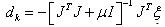
3.2.1. MLP

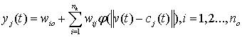
A three-layer feed forward ANN called Multi Layer Perceptron (MLP) has been applied in this paper. In the input layer, the number of nodes is corresponded to the number of input variables. The output node represents 1 and 0 for malignant lesion and benign ones, respectively. Linear and hyperbolic tangent sigmoid transfer functions have been considered as activation functions of input and hidden layers, respectively.

Gradient Descent (GD) back propagation and Levenberg-Marquardt (LM) back propagation are applied to train MLP neural network.

In GD, the value of weight update is calculated as follows:

(2)

where n is the iteration count, η is the learning rate, and p(n) is the step direction taken in the n-th iteration step[12].

Other training algorithm used in this study is LM method is reputably the fastest back propagation algorithm. It can be thought of as a combination of steepest descent and the Gaussian Newton method. At each iteration of the learning process, the weight vector w will be updated as following:

(3)

(4)

where, d_k is search direction, μ is damping parameter of k-th iteration, is a vector of network errors and J is the Jacobian matrix that contains first derivatives of the network errors with respect to the weights[13].

3.2.2. GRNN

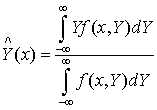
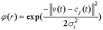
General Regression Neural Network (GRNN) is one of the neural networks applied in this paper. A GRNN can be thought of as a normalized Radial Basis Function (RBF) network in which there is a hidden unit centered at every training case. These RBF units are known as kernels and are usually probability density functions (e.g., Gaussian). The hidden-to-output weights are the target values, so the output is a weighted average of the target values of training cases close to the given input case. The following formula can be used to find the estimated value of random variable Y in any point of space X[13]:

(5)

where F (x, y) can be estimated by observing the values of x and y. Thus, the previous formula can be rewritten as

(6)

Where

(7)

The only weights that need to be learned are the widths of the each kernel, known as smoothing parameters σ. These parameters provide a smooth transition from one observed value to another, even with sparse data in a multidimensional space[13].

3.2.3. PNN

Probabilistic Neural Network (PNN) is also applied as a classifier in this paper. The probability density functions of PNN like GRNN are evaluated using the Parzen’s nonparametric estimator. PNN utilizes one probability density function for each category, as shown by (8).

(8)

Where d denotes the dimension of the pattern x, σ is the smoothing parameter and x_ij is the neuron vector[14].

The main differences between GRNN and PNN are weights connected the hidden layer to output layer. Usually, these are one or zero on PNN; for each hidden unit, a weight of 1 is used for the connection going to the output that the pattern belongs to, while all other connections are given weights of 0. The output unit performs classification according to the well-known Bayes’s theory[15].

3.2.4. RBF

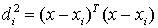
A RBF network is a one-hidden-layered feed forward neural network. The first layer consists of input nodes connected to a hidden layer via a set of unity connections, and the outputs of the input layer are determined by calculating the distance between the network inputs and hidden layer centers. A RBF network with no outputs and n_h hidden nodes can be expressed as:

(9)

Where w_ij, w_io, c_j(t), n_h and n_o are the connection weights, bias connection weights, RBF centers, number of hidden nodes and number of outputs respectively; v(t) is the input vector to the RBF network and φ(.) is a non-linear basis function. The notation ||.|| denotes a distance measure that is normally taken to be the Euclidean norm.

Typically the activation function of hidden layer unit for an input vector v is given by (10)[16]

(10)

3.2.5. SVM

The Support Vector Machine (SVM) introduced by V. Vapnik in 1995 is a method to estimate the function classifying the data into two classes[17, 18]. The basic idea of SVM is to construct a hyper plane as the decision surface in such a way that the margin of separation between positive and negative examples is maximized. The SVM term come from the fact that the points in the training set which are closest to the decision surface are called support vectors [19].When used in classification; SVM maps the input space to higher dimensional feature space and constructs a hyper plane, which separates class members from non-members [20].

Training vectors xi is mapped into a higher dimensional space by a function Ø. Then SVM finds a linear separating hyper plane with the maximal margin in this higher dimensional space. Furthermore, k (x_i, x_j) =Ø (x_i) Ø (x_j) is called the kernel functions. There are number of kernels that can be used in SVM models. These include linear polynomial, RBF and sigmoid[21]:

Linear

Polynomial

RBF

Sigmoid

where γ> 0 is a parameter that also is defined by the user [21].

3. Results

First, every feature of all lesions is normalized to have zero mean and unit variance according to (11). Forward selection algorithm is used for best feature selection. Then selected features are applied to classifiers. To obtain optimal structure of neural networks, the number of hidden units is varied from 2 to the number of input nodes. Therefore, the structure with the lowest validation error is considered as an optimal structure.

(11)

Four-fold cross validation has been applied to evaluated generated classifiers. In k-fold cross-validation method, the dataset D is randomly split into k mutually exclusive subsets (the folds) D1, D2 …, Dk of approximately equal size. The inducer is trained and tested k times each time t ∈{1, 2 …, k}, it is trained on k-1 subsets, and tested on the remaining ones [22].To evaluate the performance of neural network approach, accuracy, sensitivity and specificity of outputs are calculated. Also area under ROC (AUC) was calculated for performance comparison.

Diagnostic performance of shape, texture and kinetic features for mass, non-mass and all lesions based on forward selection, are shown respectively on Table 3, 4, 5. Selected features are presented by numbers presented in Table 2. Notice that the numbers are expressed as percentage.

Table 3. Performance of Classifiers for Mass Data Using Selected Features by Forward Selection ACC SE SP AUC Selected Feature MLP (GD) 92 98 79 94 4,6,13,15,20 MLP (LM) 83 91 63 86 17,18,19,20 RBF 76 83 64 87 4,7,10,15,20 PNN 97 100 85 – 3,6,13,14,18 GRNN 82 97 63 92 15,16,18,19,20 Linear SVM 81 90 75 – 3,9,11,19,20 Poly SVM 87 95 72 – 9,11,12,13,15 MLP SVM 85 95 68 – 9,15,17,18 RBF SVM 83 95 67 – 3,6,9,16,20

Table 4. Performance of Classifiers for Non-mass Data Using Selected Features by Forward Selection ACC SE SP AUC Selected Feature MLP (GD) 89 100 63 92 5,10,12,16,19 MLP (LM) 80 92 50 81 17,18,19,20 RBF 78 88 58 79 6,7,10,15 PNN 96 100 83 – 6,10,14,15 GRNN 84 97 25 55 7,14,15,16,20 Linear SVM 91 98 63 – 6,16,18,19 Poly SVM 91 95 69 – 6,16,18,19,20 MLP SVM 95 100 71 – 4,6,7,15,16 RBF SVM 87 100 50 – 6,7,11,18,20

Table 5. Performance of Classifiers for all Data Using Selected Features by Forward Selection ` ACC SE SP AUC Selected Feature MLP (GD) 80 82 72 76 5,10,13,15,20 MLP (LM) 81 91 57 73 16,17,19,20 RBF 77 82 56 76 5,6,7,13,15 PNN 94 100 75 – 6,8,12,15,20 GRNN 88 99 52 84 8,13,14,15,16 Linear SVM 87 96 56 – 13,14,15 Poly SVM 88 98 58 – 13,14,15 MLP SVM 84 92 68 – 3,5,11,14,18 RBF SVM 86 96 57 – 10,14,16,19

4. Discussion

Breast cancer is the most common malignancy in the world affecting the female population. The important (primary) aim of this study was to compare several classifiers and to select the best quantitative features to differentiate between malignant and benign breast lesions in patients. Using our data set of 112 lesions, including mass and non-mass-like lesions, forward selection method has been applied for the best feature selection among twenty extracted features. To classify data set into malignant and benign group, several classifiers have been applied in three group data: Mass, Non-mass and all malignant and benign lesions.

As shown in above tables, in all type of data, PNN obtained maximum accuracy among all classifiers. According to Figure 1, K^trans, sum average and entropy are the most important feature in mass group. As you see in Figure 2, sum variance is the most important feature in non-mass group. Also, circularity is significant in classification of non-mass data.

According to Figure 3, sum average, homogeneity and correlation, have the greatest number of selection in all data for classification.

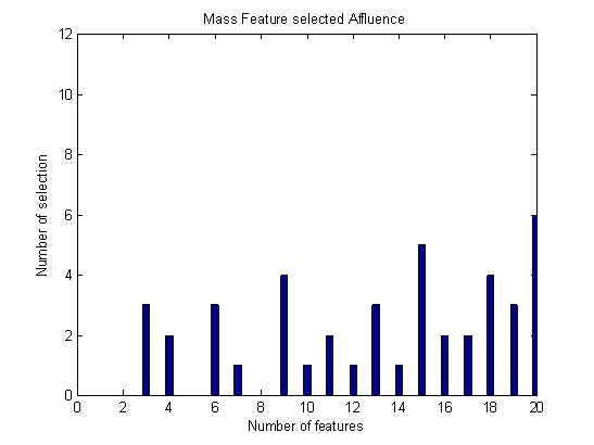Figure 1. Number of each feature selection in mass group.

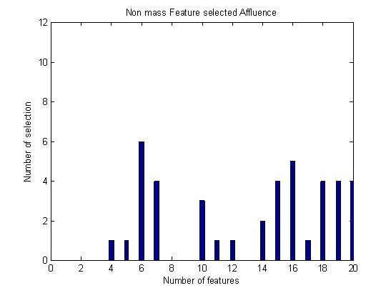Figure 2. Number of each feature selection in non-mass group.

5. Conclusions

In this study, breast cancer on dynamic MRI is classified by using forward selection and some classification methods. Appropriate quantitative parameters, can be chosen as the best features for classification based on forward selection method. MLP_NN, PNN, GRNN, RBF and SVM are applied to classify breast cancer into two groups; benign and malignant lesions. Results confirm that PNN is the best classifier among other methods for classification of these data.

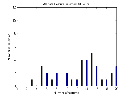Figure 3. Number of each feature selection in all data

ACKNOWLEDGEMENTS

The authors would like to thank Dr. Min-Ying Su and Ke Nie (University of California) for providing applied database in this work.