M. B. Khodabakhshi 1, H. Behnam 1, H. P. Mehrabany 2
1School of Electrical Engineering, Department of Biomedical Engineering, Iran University of Science and Technology, Narmak street, Tehran, Iran
2Faculty of Engineering, Shahed University, Khalij-e-Fars high way, Tehran, Iran
Correspondence to: H. Behnam , School of Electrical Engineering, Department of Biomedical Engineering, Iran University of Science and Technology, Narmak street, Tehran, Iran.
| Email: |  |
Copyright © 2012 Scientific & Academic Publishing. All Rights Reserved.
Abstract
This study aims to propose a computer simulation method for generating blood flow ultrasound signals. It mainly focuses on the simulation of radio frequency (RF) of moving objects in vessels, because RF signals contain more information than Doppler signal simulation. This method simulates RF signal on the basis of the acoustic field calculations. Furthermore, the resulting signal also includes Doppler Effect. The Doppler Effect is introduced while assuming the system is linear time variant (LTV). That is, when a scatterer moves, its spatial impulse response changes by time. Therefore, we could consider the desired Doppler Effect in the signals. Different velocity of a cardiac cycle is applied to the model and their corresponding frequency shifts are calculated by applying fast Fourier transform. The results of study show correct frequency shifts in the simulated signal. We further compared our simulated signal with a RF signal recorded from human aorta by a longitudinal scan. According to the results, the normalized root mean square error in one cardiac cycle between velocity profile of the simulated and experimental signals is 13.02% and that verifies the similarity of our proposed method to the real data.
Keywords:
Ultrasound, Radio Frequency, Doppler Effect, Blood Flow
Cite this paper:
M. B. Khodabakhshi , H. Behnam , H. P. Mehrabany , "Ultrasound Radio Frequency Signal Simulation Considering Doppler Effect by Use of Linear Time Variant Model", American Journal of Biomedical Engineering, Vol. 1 No. 1, 2011, pp. 1-6. doi: 10.5923/j.ajbe.20110101.01.
1. Introduction
Determination of instantaneous velocity of blood flow is a useful hemodynamic parameter which may be used to diagnose the arterial diseases such as stenosis and embolus detection. The velocity known as Doppler ultrasound technique is obtained non-invasively through diffusion of ultrasound waves into vessels. In Doppler technique, the ultrasound wave is transmitted with a certain frequency to the blood vessels from a specific angle to the vessel. Given the movement of the blood in the vessels, the frequency of returning signal will differ from that of initial transmitted signal. This is called Doppler shift. The Doppler shift, a change in the frequency of a reflected sound wave due to motion between a sound source and a reflector, was first studied by Christian A. Doppler, an Austrian physicist, in the 1800s[1]. The instantaneous velocity is ultimately extracted from the Doppler shifts.Ultrasound signal models can provide us with further knowledge of physical processes and improve our ability to design better signal analysis techniques. Different methods for simulation of ultrasound signals in human tissues were proposed. Mo and Cobbold[2] showed that Doppler signal could be synthesized on a computer using a sinusoidal model. They also illustrated that statistical behavior of the simulated Doppler signal in both time and frequency domains corresponded with the signals observed in human artery. These comparisons were made on an interval of 0.001 second on peak systole.Yu Zhang et al.[3] have proposed a Doppler simulation model in order for detecting embolus. The sample volume of their study was divided into many sub-categories in both radial and axial directions. The Doppler ultrasound signal of each sub-category was then simulated by an exponential equation. At next stage, they estimated profile of the instantaneous velocity, by using Womersley’s theory as well as updating the location of each sub-category.In another study, Wang et al.[4] proposed a simulation model to generate Doppler ultrasound signals from pulsatile blood flow in the vessels with various degrees of stenosis. They produced the Doppler signals using cosine-superposed components modulated by a power spectral density function varying over the cardiac cycle.Attending to a number of moving scatterers randomly distributed in the vessels, Hajjam et al.[5] simulated the ultrasound signal. They proposed a method which was modified in time domain. In their study, Doppler Effect has been introduced in the form of a change in the signal shape in accordance with a calculated value gained from the speed of the scatterers. As such, the simulation model is based on ‘Field II’ simulation package developed by Jensen et al.[6]. Field II is a type of software which is capable of calculating the emitted fields and echoed pulses for both pulsed and continuous wave signals for large number of different transducer geometries. The package does not take into account the Doppler shift.A brief review of previous studies indicates that few simulations have been based on the acoustic field equations and the studies mainly generate the given signal by proposing a mathematical model. Researchers have mostly focused on the simulation of Doppler signals and RF signal simulation is rarely considered[6,7]. In Field II package, the pulsed echo signal is calculated by the concept of spatial impulse responses as developed by Tupholme and Stepanishen[6]. Accordingly, RF is the resulting signal. Jensen[6] took frequent photos of scatterer’s echoes in different times for generating signals from blood flow. We know that when the signal is emitted by transducer to reach scatterers, they are actually moving. Therefore, a Doppler shift which corresponds to scatterer’s velocity must be considered in the simulation in order to produce a correct echo signal. The main purpose of our study is hence to model the returning RF signal from blood flow which includes the Doppler shift based on instantaneous velocities of scatterers. The proposed model in this study has two characteristics. First, the RF signal (instead of Doppler signal) is simulated based on the equations of ultrasound wave propagation in body tissues. Second, the Doppler Effect of the moving particles in the vessels has been appeared in resulting signal. Considering the system in the form of linear time variant (LTV), The Doppler Effect is introduced in current study. In this paper, we have initially explained our simulation method and how to generate the RF signal from acoustic field calculations. Then, LTV system considerations and the implementation of Doppler Effect are described. The FFT is applied to the simulated RF signals and it was shown that extracted values were highly similar to the initial input velocity. Finally, the comparison of a time-frequency analysis between the synthesized RF signal and the clinical RF signal has been displayed.
2. Material and Methods
2.1. The Principles of Calculating the RF Signals
We considered a disk transducer for transmitting signal. The transducer was stimulated by a hamming windowed sinusoidal signal. We consider the acoustic pressure in front of the transducer as RF signal. We used the equations of ultrasound wave propagation equations based on Rayleigh integral [8], for calculating acoustic pressure. Rayleigh integral describes the velocity potential of each point in front of an ultrasound transducer. Rayleigh integral for a transducer lay in plane Z=0 can be written as follows: | (1) |
Where is velocity potential;
  velocity waveform; and
  apodization function. Figure 1 shows the geometry of disk transducer and the location of scatterers in front of it.
 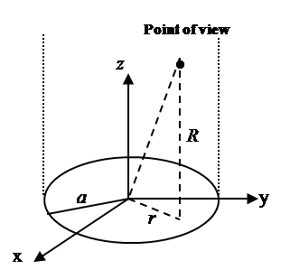 | Figure 1. A disk transducer lay in Z=0 plane. a is radius of disk transducer, z is vertical distance from the point of view to the transducer plane, and r is the distance from the center of disk transducer to the point of view’s projection in the plane of disk transducer. |
According to Cobbold[8] velocity potential and spatial impulse response are written as follow: | (2) |
 | (3) |
 | (4) |
The acoustic pressure of points in front of transducer obtains from: | (5) |
Where  is density. In accordance with equation (5), in order to obtain the acoustic pressure the impulse response for an arbitrary location from a transducer must be calculated. For simplification, the spatial impulse response has been calculated by using the Ring function, as stated by Cobbold[8].If the scatterer doesn’t have any movement, the spatial impulse response and acoustic pressure could be obtained through equations (4) and (5). The frequency of this signal is the same as exciting signal. However, if the scatterer moves, the frequency of response signal needs to differ from transmitted wave. In the described method, if we watch the scatterer at separate time intervals and calculate the responses, the frequency of response signal will not change and we will have a series of identical response curves that are slightly delayed in time. But if we take notice of the scatterer movement during the wave radiation, we can show the frequency shift pertaining to the velocity of moving scatterer. In other words, in accordance with the scatterer velocity and its updated location, the spatial impulse response at each moment could be calculated by equation (4). Then, the acoustic pressure at each moment is obtained from equation (5), depending on the overlap of the transmitted wave and the spatial impulse response. This means we have considered that the system is Linear Time Variant (LTV).
2.2. Ltv System Properties
LTV system is one which its impulse response changes by time. Therefore, the integral of linear convolution cannot calculate the system response. We should compute the system impulse response at each moment to achieve LTV system response. LTV system impulse response is displayed as  which belongs to time
  and
and  input. In other words, LTV system impulse response is obtained by applying lagged impulses at different times. The output of LTV system is calculated through the following equation:
 | (6) |
Where  and
and  are input and output signals;
  is LTV system impulse response; and
  the is the time when impulse
  is applied.Figure 2 illustrates the stages of calculating a moving scatterer’s response in front of a disk transducer. At each moment the scatterer and transmitted wave are subsequently transferred to new locations on the basis of their velocities. So the spatial impulse response and the acoustic pressure corresponding with new locations are calculated and the system output for each moment is consequently computed. The calculations are stopped once the transmitted wave passes from the scatterer.
3. Experiments and Results
A disk transducer with a 1cm radius for transmitting a 3.2 MHz signal is used in the current study. Figure 2 shows the transducer location in relation to the scatterer in simulation. For exciting the transducer, a 3.2MHz sinusoidal signal which is multiplied to a Hamming window has been used. Sound velocity in tissue is 1540m/s. Because of the scatterer velocity is to a large extent lower than the sound velocity and we should find the very small frequency differences between the transmitted wave and the scatterer signal, sampling rate from 100MHz to 1GHz and a ten-million points FFT for validation are considered. These frequency differences are about 100-1000Hertz as opposed to several mega Hertz. If the values of sampling frequency are smaller than those expressed, the transmitted wave will quickly pass the scatterer and the Doppler effect cannot appear in the final signal. Furthermore it is impossible to extract the frequency differences, when the FFT points were less than ten million.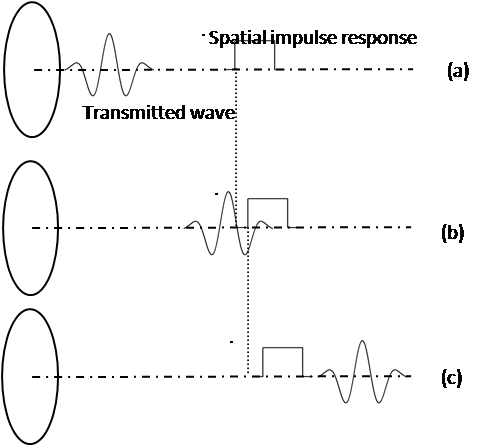 | Figure 2. Calculating the acoustic pressure of a moving scatterer in front space of disk transducer. When signal is emitted by the transducer, the scatterer actually moves and the system’s spatial impulse response changes. (a) The transmitted wave has not reached scatterer location. (b) The transmitted wave has hit scatterer. (c) The transmitted wave has passed the scatterer. |
Figure 3 shows the results of simulation for a moving scatterer with 47cm/s velocity and its FFT diagram in comparison to a fixed scatterer. The corresponding frequency shift can be seen in Figure 3.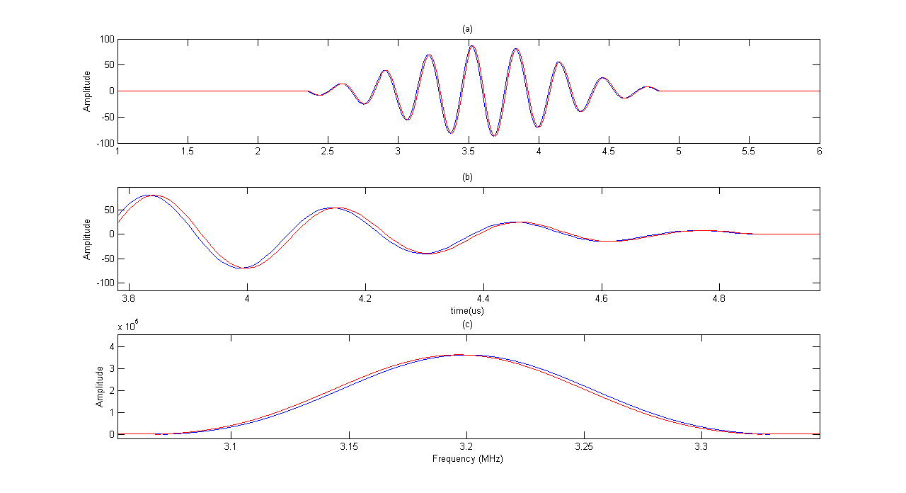 | Figure 3. Moving scatterer signal (red line) versus fixed scatterer signal(blue line). (a)moving and fixed scatterers RF signals (b) close up shows of RF signals (c) Their corresponding FFT diagram. The moving scatterer spectrum has slightly shifted to left. |
After applying FFT, we used the following equation to see if the velocity of simulated signals matches with the initial input velocity[1]: | (7) |
Where,  is transducer central frequency;
  Doppler frequency shift; c sound velocity; and V scatterer velocity. Table 1 shows the results of experiment for scatterers with different velocity as input and also the velocity obtained from FFT and equation 7. The results indicate high accuracy in generating RF ultrasound signals in vessels.
| Table 1. The estimated velocity gained from applying FFT to simulated signal |
| | Applied Velocity (cm/s) | Estimated velocity (cm/s) | | 24 | 23.099 | | 35 | 34.648 | | 47 | 46.2 | | 50 | 50.0047 | | 62 | 61.597 | | 80 | 80.846 | | 110 | 107.8 | | 150 | 150.14 | | 175 | 173.24 | | 200 | 200.19 |
|
|
4. Discussion
It has been shown that it is possible to consider Doppler effect in the final RF signal using a LTV model. We used an ultrasound RF signal recorded from a 33 years old healthy man’ aorta in the longitudinal scan by a B-K Medical A/S type 3535, to indicate that our synthesized RF signal is similar to those found in practice. Table 2 exhibits the specifications of this practical RF signal which is downloaded from(http://server.elektro.dtu.dk/ftp/jaj/31655/ult_data/in-vivo/rf_data/).From Table 2 it can be understood that a 2 mm gate in the aorta is exposed 3500 times per second and 2.28 seconds of RF signal lines (8000 lines) are obtained. Figure 4 shows some of those RF lines. 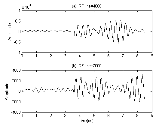 | Figure 4. Some of recorded RF lines: (a) 4000th line; (b) 7000th line. The data is used in 3.7 to 8.53 µs. |
At this stage, we should extract the velocity profile calculated from the frequency shift. The purpose of this stage is to apply the experimental signal velocity profile as an input into our model and finally to compare both signals together. We used ‘Slow Time’ method for extracting frequency shift[8]. If we expose the vessels to a specific pulse repetition frequency (PRF) and study all the received RF signals in a fixed instant of time, the overall shape of the transmitted pulse can be reconstructed which is called ‘Sampled Amplitude’. The time interval between samples is . The particle velocity element is proportionate with the central frequency of the sampled amplitude waveform which is computed by equation (7).
| Table 2. The specifications of recorded signal from a 33 years old man |
| | Transducer | B-K 8556, 3.2 MHz linear array probe | | Pulse repetition frequency | 3.5 kHz | | Sampling frequency | 15 MHz | | Depth | 50 mm | | Range gate | 2 mm | | RF lines | 8000 | | Samples per line | 128 |
|
|
Therefore, we applied slow time method to the practical RF lines and the sampled amplitude related to time 6.5µs is shown in Figure 5. This figure contains 2.28s of data and its corresponding spectrogram. It can be seen that the spectrogram contains 3 peaks of systole presented in time interval. The velocity profile obtained from the experimental data spectrogram, and also the specifications mentioned in Table 2 are fed into our simulation model. In order to generate comparable simulation data to experimental data, we put a scatterer in front of the transducer at its 5cm distance and monitored its movement with different velocity extracted in one second from experimental spectrogram. Therefore, 3500 RF lines were produced and a cardiac cycle was obtained. At a fixed instant of time, we investigated all simulated RF lines signals and made the waveform of sampled amplitude range by slow time method. Then, the spectrogram of this waveform was achieved.Figure 6-a, 6-b are the spectrogram of simulated signal versus the experimental signal which are obtained by the slow time method. The figures show the low frequency components in the experimental data which does not emerge in simulated data spectrum. We used the mean velocity profile of the experimental data which is not containing the low frequency components as an input of our model (Figure 6-c). Due to lack of these low frequency components in the Figure 6-c, they are not appeared in the simulated signal spectrogram. This Figure 6 verifies the similarity between the spectrum analysis of both experimental and synthesized signals. To quantifying the differences between velocity values predicted by our model and experimental velocity values we used the Normalized Root Mean Square Error (NRMSE) according to equation (8): | (8) |
Where  and
and  are the time-varying mean velocities of clinical and synthesized signals. The velocity profile of both signals is shown in Figure 6-c and 6-d. The NRMSE was 13.02% for our proposed model.
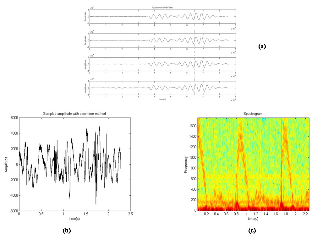 | Figure 5. Slow time method has been applied to experimental data. (a) Four successive RF lines. (b) Sampled amplitude at a fixed instant time. (c) Spectrogram of sampled amplitude (instantaneous Doppler shifts). |
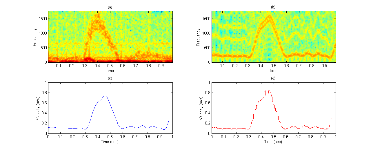 | Figure 6. Comparison of practical data and our simulated data: (a) practical data spectrogram; (b) simulated data spectrogram; (c) velocity profile extracted from experimental data and fed to the model; (d) velocity profile extracted from simulation data. |
5. Conclusions
A new method is introduced for simulation of ultrasound RF signal containing Doppler Effect. In this study we focused on the simulation of RF instead of Doppler signal. It can be concluded that, the described method in current study can express a real ultrasound signal which is scattered from the moving particles in vessels. The calculations of spatial impulse response had been previously applied in Field II for simulation of fixed tissues in body. However, the method of spatial impulse response is not solely sufficient if we want to simulate blood flow signal, because the frequency shift corresponding to scatterer velocity will not appear. We assumed the system as linear time variant. Therefore, the aforementioned spatial impulse response changes by time and we should calculate the RF echo signal at each moment based on its own impulse response. The Doppler shift was thus considered in our method. The results showed that the synthesized signal through given velocity profile is greatly consistent with the practical signal. We intend to simulate embolic signals through this model, in order for further use of it. When an embolus passes a vessel, a stochastic signal with high amplitude and transit time is produced in RF echo signal which also affects the velocity profile. Finally, the model can be used as the signal simulator of Trans Cranial Doppler (TCD).
References
| [1] | T. J. DuBose, A. L. Baker, Acoustic Doppler shifts in medicine, Applied Acoustics.68 (2007) 240–244 |
| [2] | L. Y. Mo, R.S.Cobbold, Speckle in continuous wave Doppler ultrasound spectra: A simulation study, IEEE Trans. Ultrason., Ferroelect., Freq. Contr.UFFC-3 (1986) 747-753. |
| [3] | Y. Zhang, H. Zhang, N. Zhang, Microembolic signal characterization using adaptive chirplet expansion, IEEE Trans. Ultrason., Ferroelec., Freq. Contr. 52 (2005) 1291-1299. |
| [4] | L. Wang, Y. Zhang, D. Wang, N. Su, C. Du, A Simulation Model for Doppler Ultrasound Signals from Pulsatile Blood Flow in Stenosed Vessels, international conference on biomedical eng and informatics (2008) |
| [5] | A. Hajjam, H. Behnam, A modified time-domain approach for modeling the ultrasound signal from blood-flow" Ultrasound. 16, (2008) 160–164 |
| [6] | J. A. Jensen, N. B. Svendsen, Calculation of pressure fields from arbitrarily shaped, apodized, and excited ultrasound transducers. IEEE Trans. Ultrason., Ferroelec., Freq. Contr. 39 (1992) 262–267 |
| [7] | MB. Khodabakhshi, H. Behnam, A New Method for Simulation of Embolic Signal in Ultrasound Blood Flow Signals (A TCD Simulation), Proceedings of the 17th Iranian Conference of Biomedical Engineering (ICBME2010), 3-4 November 2010 |
| [8] | RS. Cobbold. Foundations of ultrasound, Toronto: Oxford Press, 2007 |
| [9] | J. A. Jensen. Field: A program for simulating ultrasound systems. Med. Biol. Eng. Comp., 10th Nordic-Baltic Conference on Biomedical Imaging, Vol. 4, Supplement 1, Part 1:351–353, (1996) |
| [10] | R. Zahiri-Azar and S. E. Salcudean, “Motion estimation in ultrasound images using time domain cross correlation with prior estimates,”IEEE Trans Biomed Imag, vol. 53, no. 10, pp. 1990–2000, (2006) |
| [11] | F. Viola and W. Walker, “A spline-based algorithm for continuous time-delay estimation using sampled data,” IEEE Trans Ultrason Ferroelectr Freq Control, vol. 52, pp. 80–93, 2005. |
| [12] | P. R. Stepanishen. The time-dependent force and radiation impedance on a piston in a rigid infinite planar baffle. J. Acoust. Soc. Am., 49:841–849, (1971) |
| [13] | P. R. Stepanishen. Transient radiation from pistons in an infinite planar baffle. J. Acoust. Soc. Am., 49:1629–1638,(1971) |
| [14] | D.Evans, Ultrasonic Detection of Cerebral Emboli, IEEE Ultrasonics Symosium,(2003) |
| [15] | E.O.Kung,A.S.Les,A.Figuera,In Vitro Validation of Finite Element Analysis of Blood Flow in Deformable Models, Annals of Biomedical Engineering, Vol. 39, No. 7, (2011) pp. 1947–1960 |
| [16] | J.Cowe, J.Gittins, A.Naylor, D.Evans, RF Signals Provide Additional Information on Embolic Events Recorded During TCD Monitoring, Ultrasound in Med. & Biol., (2005), Vol. 31, No. 5, pp. 613–623 |
| [17] | Rainer Brucher, David Russell,” Automatic Online Embolus Detection and Artifact Rejection With the First Multifrequency Transcranial Doppler” Stroke Journal of the American Heart Association, April 16, 2002 |
 Abstract
 Reference
 Full-Text PDF
 Full-Text HTML