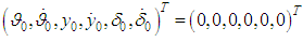
-
Paper Information
- Paper Submission
-
Journal Information
- About This Journal
- Editorial Board
- Current Issue
- Archive
- Author Guidelines
- Contact Us
International Journal of Aerospace Sciences
p-ISSN: 2169-8872 e-ISSN: 2169-8899
2017; 5(1): 8-23
doi:10.5923/j.aerospace.20170501.02

Modeling of Transition Processes in a Partially Invariant Center of Mass Motion Stabilization System
 Abstract
 Reference
 Full-Text PDF
 Full-text HTML
Nickolay Zosimovych
Intelligent Manufacturing Key Laboratory of Ministry of Education, Shantou University, Shantou, China
Correspondence to: Nickolay Zosimovych, Intelligent Manufacturing Key Laboratory of Ministry of Education, Shantou University, Shantou, China.
| Email: |  |
Copyright © 2017 Scientific & Academic Publishing. All Rights Reserved.
This work is licensed under the Creative Commons Attribution International License (CC BY).
http://creativecommons.org/licenses/by/4.0/

The publication suggests how to significantly improve the spacecraft centre of mass movement stabilization accuracy in the active phases of trajectory correction during interplanetary and transfer flights, which in some cases provides for high navigation accuracy, when rigid trajectory control method is used. The required stability conditions obtained are consistent with the known criteria in the invariant theory. Computer modelling shows that in a partially invariant stabilization system reveals the significant advantages of such a system in terms of greater accuracy when compared to known stabilization systems.
Keywords: Space vehicle (SV), Stabilization controller (SC), On-board computer (OC), Gyro-stabilized platform (GSP), propulsion system (PS), Angular velocity sensor (AVS), Operating device (OD), Feedback (FB), Control actuator (CA), Control system (CS), Angular stabilization (AS), Centre of mass (CM)
Cite this paper: Nickolay Zosimovych, Modeling of Transition Processes in a Partially Invariant Center of Mass Motion Stabilization System, International Journal of Aerospace Sciences, Vol. 5 No. 1, 2017, pp. 8-23. doi: 10.5923/j.aerospace.20170501.02.
Article Outline
1. Introduction
- The thriving space technology is characterized by an increasing complexity of the tasks to be solved by modern space vehicles (SV). The efficiency in solution of such tasks significantly depends upon technical characteristics of the on-board systems ensuring the functioning of the spacecraft. In some cases, when using a control system built according to the principle of program control (the "robust trajectories" method) the efficiency of task solution is much influenced by the accuracy of the spacecraft stabilization system in the powered portion of flight. This concerns, for example, the trajectory correction phases during interplanetary and transfer flights, when the rated impulse execution errors during trajectory correction resulting from various disturbing influences on the spacecraft in the active phase, greatly affect the navigational accuracy. Hence, reduction of the cross error in the control impulse on the final correction phase during the interplanetary flight, facilitates almost proportional reduction of spacecraft miss in the "perspective plane". For example, in some space probes (SP) like Deep Impact [1, 2] and Rosetta missions [3, 4] reduction of cross error by one order during the execution of correction impulse (for modern stabilization systems this value shall be results in reduction of spacecraft miss in the "perspective plane" from 200 to 20. Such reduction of the miss accordingly increases a possibility of successful implementation of the flight plan, as well as the accuracy of the research and experiments conducted [5].The Martian Moons Exploration (MMX) mission is scheduled to launch from the Tanegashima Space Centre in September 2024. The spacecraft will arrive at Mars in August 2025 and spend the next three years exploring the two moons and the environment around Mars. During this time, MMX will drop to the surface of one of the moons and collect a sample to bring back to Earth. Probe and sample should return to earth in the summer 2029 [6].Besides improvement of the navigational accuracy, reduction of spacecraft stabilization cross errors in the active phase, it also results in lower total characteristic velocity of corrective impulses, and, consequently, in reduction of fuel required for the correction. So, when the correction speed impulse reaches 30 reduction of gross error during the correction manoeuvre results in proportional reduction of the required characteristic velocity during the next correction. The data referred to in [7, 8] show that improved accuracy of roll stabilization in the active phase by one order results in reduction of total characteristic correction velocity for Mars interplanetary probe (Mars-96, Russian Federation) from about 20 to 2 which corresponds to fuel savings approximately by 30, or to increase of the payload mass by 4 Due to the relatively small weight of modern scientific instruments (about 3-8), even such seemingly small increase of payload weight can significantly extend the program of research and experiments implemented by the spacecraft.Objectives: to solve the task of significant increase in stabilization accuracy of centre of mass tangential velocities during the trajectory correction phases when using the "rigid" trajectory control principle. Since the time of the active phase in correction manoeuvres, which is to be determined by the required velocity impulse, shall not be clearly determined in advance, and quite limited, and because a guaranteed approach enabling to estimate the accuracy, is always used in practice for solving the targeting tasks, we shall understand the maximum dynamic error of the transition process as concerns the drift velocity of the spacecraft to mean the accuracy of the spacecraft centre of mass movement stabilization [9].Subject of research: The centre of mass movement stabilization system in the transverse plane, which is used during the trajectory correction phases.In order the control actions could be created during the spacecraft trajectory correction phase, a high-thrust service propulsion system with a tilting or moving in linear direction combustion chamber shall be used.Functioning of the spacecraft movement stabilization channel in the transverse plane is based on the feedback principle, and together with the spacecraft this channel forms a closed deviation control system. We can consider two channels in this control system: an angular stabilization channel and centre of mass movement stabilization channel (Fig. 1).
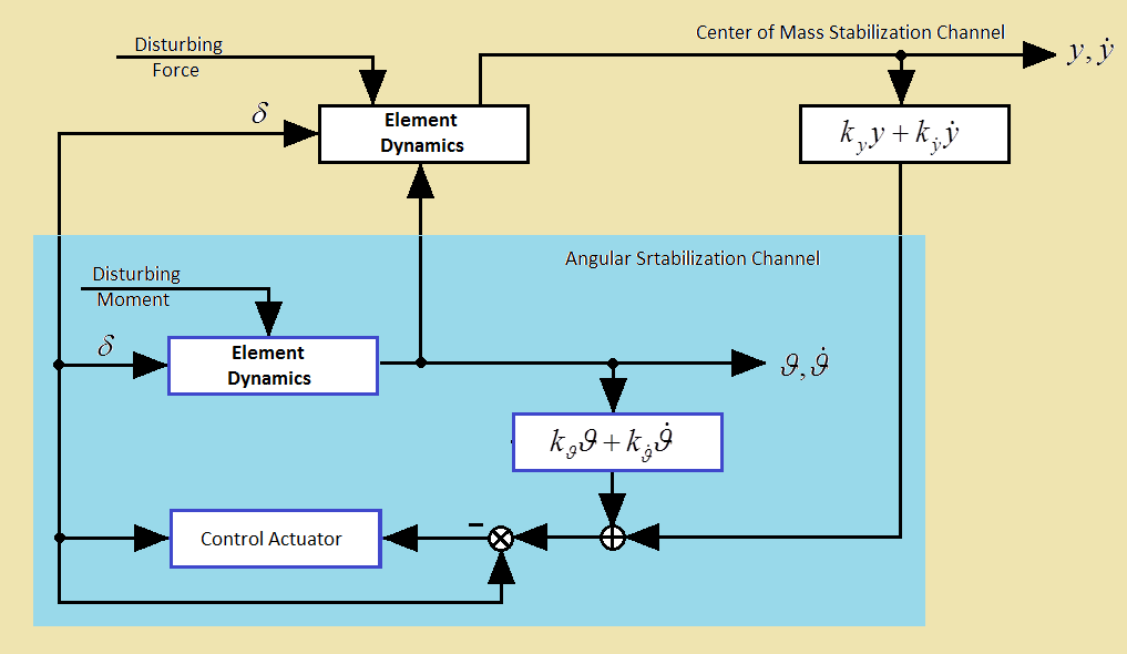 | Figure 1. Functional diagram of model spacecraft stabilization |
 and its integral-linear drift
  . In the angular stabilization channel, the control signal shall be generated in proportion to the spacecraft deviation angle in the transverse plane
  and the angular velocity of the spacecraft rotation in this plane
  .The required dynamic accuracy of stabilization of tangential velocities in this system shall be achieved through the choice of the gain in the stabilization controller
  . If the requirements to the accuracy of centre of mass movement stabilization are stiff, the coefficients
  and
and  shall be necessarily significantly increased [10]. However, if these coefficients are increased up to desired saturation, the system shall loose its motion stability, and further improvement of the accuracy of the spacecraft centre of mass movement stabilization shall be impossible when this method of control is applied. This can be explained by the fact that the increase in the gain values in the centre of mass movement stabilization channel results in improved performance of the channel, and the frequencies of the processes occurring in it become close to the frequencies of the angular stabilization channel, which fact enhances interaction of these two channels and makes it impossible to significantly improve the stabilization accuracy of the spacecraft centre of mass tangential velocities in the control system concerned.To improve the correction accuracy, the following additional algorithm shall be used in practice [12, 13]. The position of the steering control (turning PS) at the end of the previous active phase shall be memorized and set in its original position before PS is activated during next correction. The improvement of accuracy in this case shall be achieved by partial compensation of the main disturbing factors: eccentricity and thrust misalignment in the propulsion system already in the initial moment of operation of the propulsion system. This algorithm is based on the assumption that eccentricity and thrust misalignment in PS change slightly towards the end of the active phase during the previous correction, and PS setting before a new active phase sets in progress, ensures that the thrust vector goes approximately through the centre of mass of the spacecraft, thereby considerably offsetting the disturbing moment. A similar algorithm was applied in the stabilization system of the Apollo spacecraft [14]. For its implementation, the control system was complemented with a so-called compensation circuit of thrust misalignment influence. The purpose of the referred circuit was to form a component to offset the total control signal so that the thrust vector could pass approximately through the centre of mass at zero output signals from the correction filter.The stabilization systems of Titan IIIC, Kosmos-3M launchers also used subsystems tracking the centre of mass positional history, and providing the thrust vector's passage through the centre of mass [15].It should be pointed out that the process of implementation of the described algorithm is confronted by a number of challenges [16]:• Difference in disturbing factors (moments and forces) during the previous and subsequent corrections results in additional errors in the stabilization of the tangential velocities of the spacecraft centre of mass.• Due to the limited time of the active phase, deactivation of PS during the previous correction may occur even before the completion of the transition processes in the stabilization system, and as a result, the system will remember the deviation of the steering control, which was not final.Besides introduction of additional control algorithms, there are other ways to increase the accuracy of the centre of mass movement stabilization. It is a commonly known fact that one of the ways to achieve high accuracy in automatic control systems, is to use the so-called invariant theory [17-19]. The theory was developed by G.V. Shchipanov (1939), a Soviet scientist, who formulated the task "on compensation of external disturbances" [20]. Now, thanks to research conducted by the Soviet scientists G.V. Shchipanov, B.N. Petrov, V.S. Kulebakin, A.I. Kukhtenko and others the invariant theory represents a developed approach in the general theory of automatic control [16].One of the problems inherent in the synthesis of invariant control systems, is the ability for the implementation of such systems in most cases through the use of the deviation control principle, as the simplest one and most widely used in practice. The publications [21-24] consider the possibility of constructing an invariant deviation control system with one adjustable parameter including an inertial element and a servo control with feedback. The general provisions of the invariant theory prove that no absolutely invariant system can be implemented in this case because this requires that the circuit with feedback should have an infinitely great gain.As a rule, most invariant control systems are based on the use of the information about external influences. Such control systems belong to the class of combined regulatory systems. In particular, the combined systems constitute the majority of invariant systems [25-31].There is still another method to enforce implementation of invariance conditions without application of combined regulatory techniques [32]. This method is based on the dual-channel principle, which means that in order to ensure the absolute invariance of some adjustable value towards external influence, invariance with respect to the above influence should be ensured between the point of influence application and the measuring point. To implement such a system, it is necessary that two influence distribution channels should be present in the controlled element.However, the referred task, i.e. stabilization of the spacecraft centre of mass movement in the active phase provides no possibility to measure disturbing influence, and the two influence distribution channels exist in the controlled element only for one of the disturbances, namely, for the disturbing moment. Therefore, this publication proposes a way to build a highly accurate stabilization system. We suggest that the requirements to comply with the conditions of invariance should be replaced with conditions of partial invariance when considering implementation of the invariance system. This method shall enable the synthesis of a highly accurate stabilization system, where the drift velocity of the spacecraft is a partially invariant value in respect to the disturbing moment and forces influencing the spacecraft in flight. The concept of partial invariance in this case means that the invariance conditions for drift velocity shall be met regarding external influences themselves, and not their derivatives.Meeting the conditions of partial invariance significantly reduces interaction between the angular stabilization channels and the centre of mass movement stabilization channel, which is present in the known (applied in practice) stabilization systems [15, 31, 33-38] and does not allow significant improvement of stabilization accuracy of the spacecraft drift velocity.In order to improve the accuracy of the synthesized algorithms, we propose the application of self-configuring elements, which turn the operating device and X-axis of the spacecraft at angles recorded at the end of the previous active phase before a new active phase begins. The use of the above self-configuring elements in the synthesized invariant algorithms produces the maximum effect in increasing of the dynamic accuracy of tangential velocities stabilization as compared to similar techniques in the existing systems. This is due to the fact that the dynamic error of drift velocity in the synthesized algorithms, shall be largely determined by the initial conditions of the transition process due to the partial invariance of the algorithms proposed, which with the help of the mentioned self-configuring elements, can approach the values corresponding to the established mode as close as possible.The publication provides analysis of stability of the synthesized control algorithms, proves availability of stability margins in partially invariant systems sufficient for practical implementation [16]. We propose an algorithm for selection of parameters of the stabilization controller, which facilitates minimization of maximum error during stabilization of the tangential velocity of the spacecraft centre of mass while ensuring adequate stability margins in the system.
2. Modeling of Transition Processes
- This chapter provides a description and results obtained from modelling of transition processes in a synthesized partially invariant centre of mass motion stabilization system of a spacecraft (Fig. 2) and, for comparison, in a stabilization system selected as a standard one (Fig. 3).
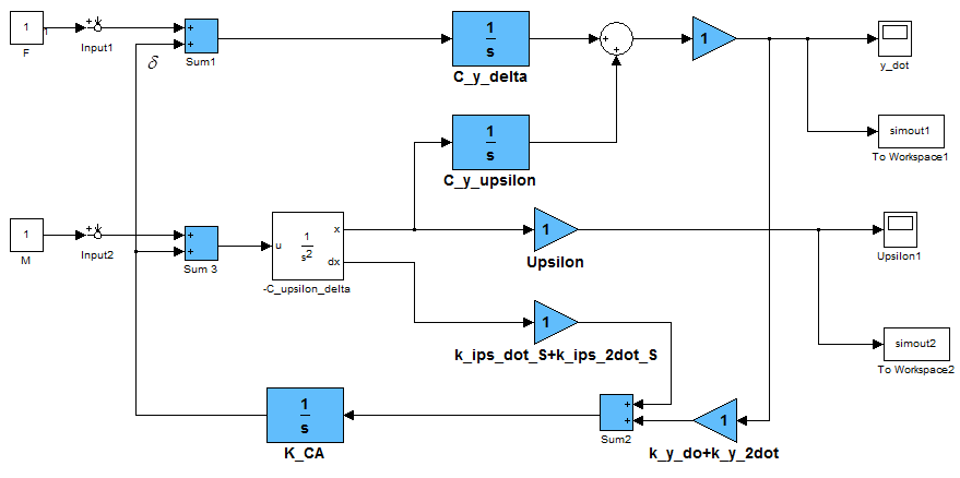 | Figure 2. Block diagram of a partially invariant centre of mass stabilization system |
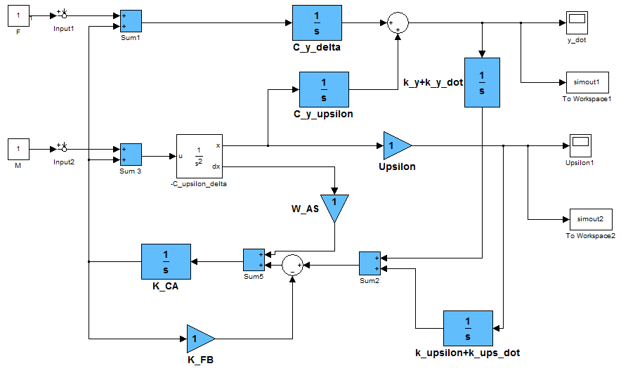 | Figure 3. Block diagram of a standard centre of mass motion stabilization system of a spacecraft |
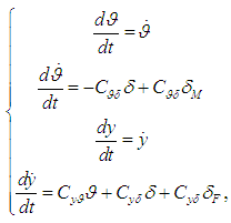 | (1) |
 are disturbances specified in the equivalent PS deviation angles. The characteristics of the test spacecraft shall be the values of the dynamic coefficients:
 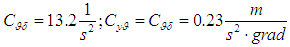 .• PS servo control: PS servo control consists of a control actuator with an open feedback (in compliance with invariance requirements) and of a current amplifier for the control actuator. The velocity performance of the control actuator has a dead zone and a saturation zone. Deviation of the operating device has limits
  on both sides from the neutral position. The current amplifier of the control actuator has a lag equal to 0.01 s. The broken feedback of the control actuator may result in the so-called 'shunt running' (a spontaneous deviation) of the control actuator. In the model, this factor shall be taken into account by supply of a continuous signal to input of the control actuator, which is 5 per cent of the value of the velocity performance saturation current in the control actuator. Consequently, PS servo control can be described by the following differential equations:
 | (2) |
 is a time constant of the current amplifier;
  is a current amplifier coefficient;
  is control voltage signal in the output of the stabilization controller;
  is amplifier-exit amperage;
  is dead band current and saturation current of the control actuator velocity performance. The following values are taken to simulate performance of the servo control:

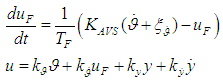
 .• Stabilization controller: Pursuant to invariance and stability conditions obtained from the synthesis of the invariant system, a stabilization expression shall be as follows:
 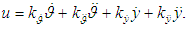 However, the expression above does not take into account several factors which, in the actual implementation of the system in question, can have a significant impact on the stabilization process, so they are to be taken into consideration when making a model. One such factor is that the second spacecraft angular deflection derivative
  has to be obtained by numerical differentiation of the signal from the angular velocity sensor (AVS) performed by the on-board computer.As a result of this differentiation, computational errors occur. In addition, calculation of the second angular derivative in the on-board computer results in delayed signals in the angular stabilization channel. AVS output signal interruptions (noise) may significantly influence the stability of the system in question, as the interruptions increase manifold during the signal differentiation. In practice, in order to partially suppress AVS exit interruptions, we use an analogy filter, which may be described by an aperiodic link of the first order with a time constant
  . However, such a filter produces signal delay in the angular stabilization channel in addition to interruptions reduction, thereby worsening the system's stability.Based on these comments, it is possible to create a system of equations that best describes operation of the stabilization controller:
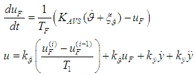 | (3) |
 is AVS filter exit signal;
  is AVS amplification factor;
  is AVS signal random error (interruption);
  is AVS filter time constant;
  are AVS signal values in the current and previous steps in calculation of a derivative from the angular velocity by the on-board computer;
  is a step in calculations of angular velocity derivative. The following values of the above characteristics were selected for modelling:
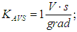


 The AVS signal error
  is considered to be Gaussian uncorrelated random value, with a zero mathematical expectation and mean square deviation (MSD)
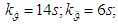
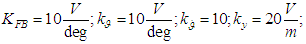
  . The MSD value was chosen from the condition that the accuracy of modern AVS is about one hundredths degree per second. The values of the stabilization controller coefficients
  were selected based on the author's algorithm.• Disturbing effects. In the model (Fig. 4), the destabilizing force and disturbing moment shall be specified in the form of equivalent deviations of the operating device
  at the exit of the corresponding elements. This takes into account disturbance changes at the moment PS starts. For high-thrust space chemical engines, normal operation mode shall be activated during the lag time
  . During "software" PS launches [39], thrust and therefore, disturbance values connected with PS operation, shall change nearly linearly from zero to those corresponding to the normal PS operating mode. In the active phase, after PS enters normal operation mode, there are slight random fluctuations in the PS operation characteristics as compared to their nominal values, which shall in its turn affect the behaviour of the disturbing effects.
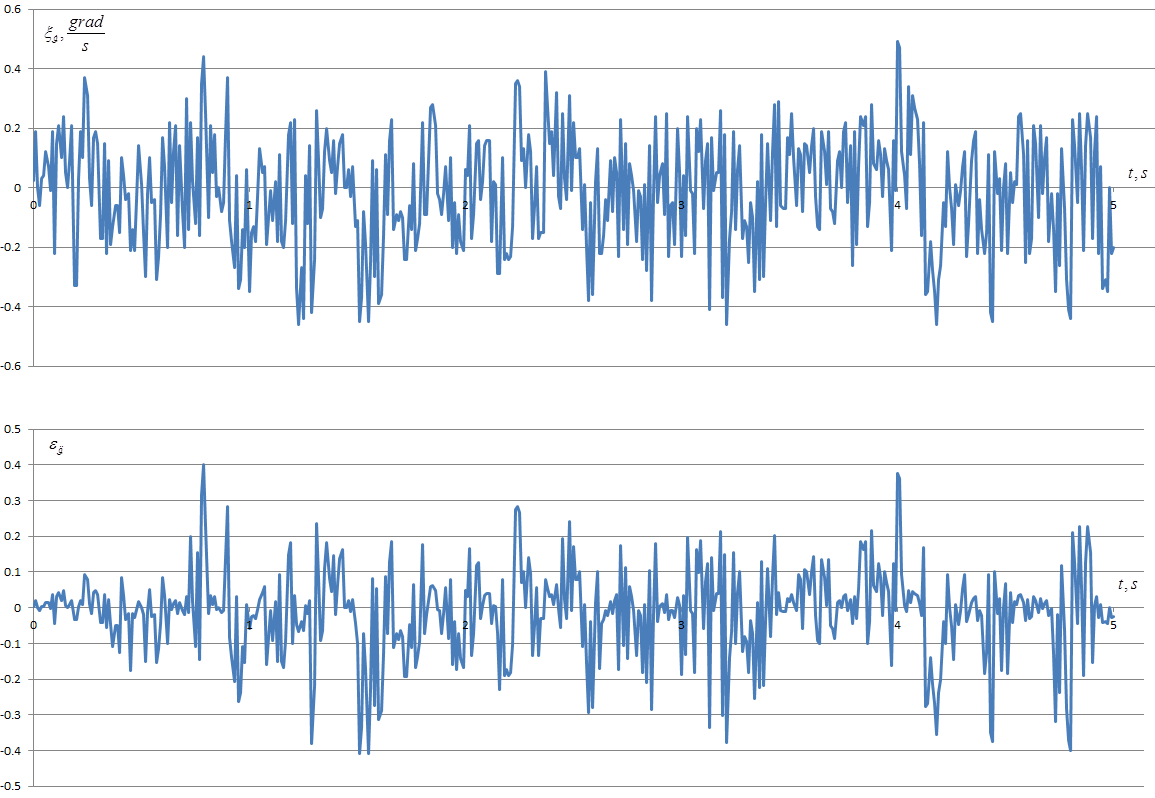 | Figure 4. Signal indicating AVS error  and the relative signal error in the derivative of angular velocity and the relative signal error in the derivative of angular velocity  as compared to the true value as compared to the true value  |
 appear as Gaussian stationary processes with mathematical expectations
  and correlation functions
 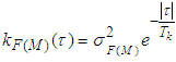 , where
  is a mean square deviation of the destabilizing force and disturbing moment in the equivalent angles of the operating device;
  is a constant, which characterizes disturbance modifications.According to [39-42], the correlative function described above has a correspondent stochastic equation or a generating filter equation of the first order:
 | (4) |
 is intensity of the white noise.The mathematical expectations of the disturbing effects shall be determined by changing PS parameters in the normal operation mode.
 | (5) |
 are the mathematical expectations disturbances in the normal operation mode of PS.The following values of the disturbance characteristics were selected for modelling:
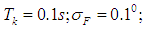

 Fig. 5 shows how disturbing effects may be realized as accidental processes.
 | Figure 5. Random modification realizations of the disturbing moment M and destabilizing force F in mathematical modelling  |
 according (4) shall be as follows:
  where
where 
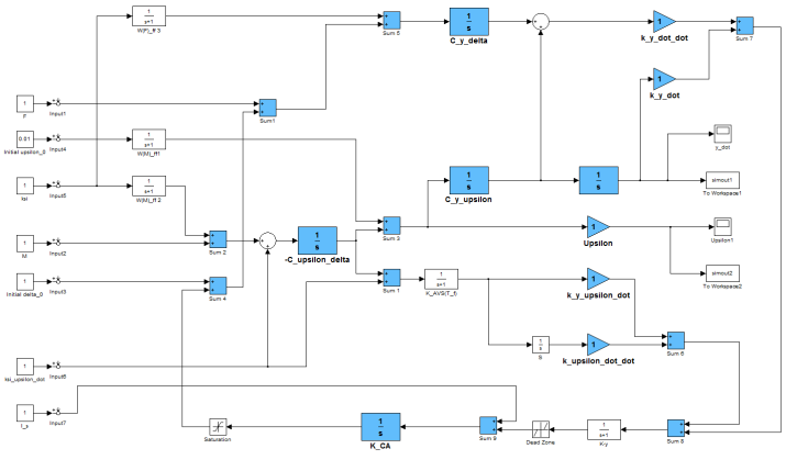 | Figure 6. Block diagram of a partially invariant centre of mass stabilization system used in the mathematical modelling |
 During the integration, the maximum drift velocity
  , was recorded, which, according to the task in question, is an indicator of the accuracy of the system. As
  is a random value because of the randomness of the disturbances, we calculated the mathematical expectation
  of this parameter and its MSD
  considering 50 realizations of the stabilization process.In order to do a comparative analysis of the stabilization accuracy in the invariant and in standard stabilization systems, similar mathematical modelling was done for the standard system as well. As appears from the block diagram (Fig. 3), presence of control actuator feedback and a different stabilization controller distinguishes a model of the standard stabilization system from the model of the invariant system. Therefore, the expressions (2) and (3) for the standard system shall be (6) and (7) respectively:
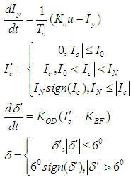 | (6) |
 | (7) |
 A block diagram for a model of the standard stabilization system used in the simulation is presented at Fig. 7.
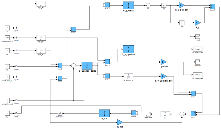 | Figure 7. Block diagram of a standard spacecraft centre of mass stabilization system used in the mathematical modelling |
 , which are in line with the situation in which most of the known, practice-based stabilization systems operate. Also we modeled a system version, which used the suggested self-regulation elements, which involves setting of the initial values according to deviations of the operating device and of the body of the spacecraft recorded at the end of the previous active phase
 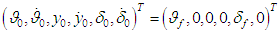 . Let's consider and analyze modeling results in each of the cases described above.
3. Zero Initial Conditions Case
- The results of the transition process modelling for the case of zero initial conditions are presented in Table 1 as mathematical expectation values
 and the mean square deviation
  of the maximum drift velocity error depending on the mathematical expectation of the disturbing effects
  .
.
|
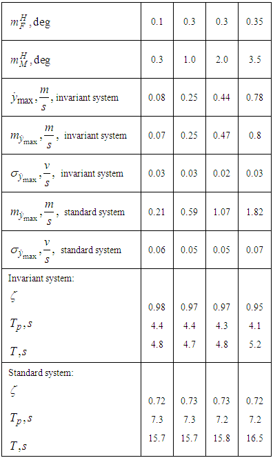
 , where
  are drift velocity amplitudes at the beginning and at the end of the period;
  is oscillation period;
  is transition process decay time. In order to assess the impact of accidental factors upon the stabilization accuracy, drift velocity stabilization error values
  , calculated according to the deterministic model of the invariant stabilization system shall be given.As the mathematical modelling shows, application of the invariant algorithm in this case improves the accuracy of centre of mass roll stabilization twice or three times. Transition processes in the invariant stabilization system have significantly less attenuation time than in the standard system. Random disturbances caused by fluctuating PS operating conditions during normal operation, as well as random AVS measurement errors in have no significant impact on the stabilization accuracy.
4. Self-Regulation Elements Version
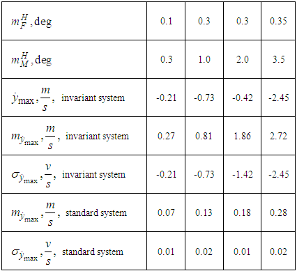
- In this case, modelling was like in the previous case, the difference being that the initial values were set non-zero
 that is we simulated initial OD and spacecraft X-axis alignment based on result of the previous adjustment (Table 2). The corresponding parameter values at the end of the transition processes were used as values
  for the case of non-zero initial conditions with correspondent
  Because in practice similar OD alignment shall be done with an error, which is approximately 30% of the true value, we used values
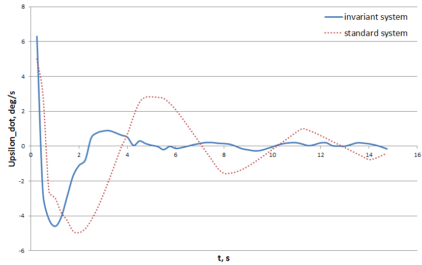
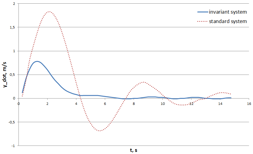
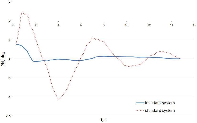
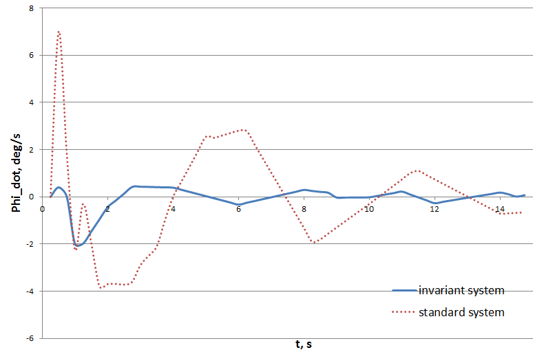
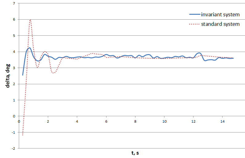
  with 30% margin of error in the mathematical modelling as well (See Fig. 8 – 15).
|
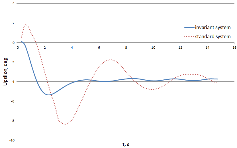
 | Figure 8. Spacecraft drift velocity transition processes in the normal plane in the invariant and standard stabilization systems  |
 | Figure 9. Spacecraft X-axis angular deviation transition processes in the normal plane in the invariant and standard stabilization systems 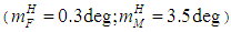 |
 | Figure 10. Spacecraft X-axis deflection rate transition processes in the normal plane in the invariant and standard stabilization systems  |
 | Figure 11. Operating device angular deviation transition processes in the normal plane in the invariant and standard stabilization systems  |
 | Figure 12. Spacecraft drift velocity transition processes in the invariant and standard stabilization systems  |
 | Figure 13. Spacecraft X-axis angular deviation transition processes in the normal plane in the invariant and standard stabilization systems  |
 | Figure 14. Spacecraft X-axis deflection rate transition processes in the normal plane in the invariant and standard stabilization systems  |
 | Figure 15. Operating device angular deviation transition processes in the normal plane in the invariant and standard stabilization systems  |
 Based on the presented results, we can conclude that the accuracy of the invariant stabilization system increases significantly and is 4-5 times higher than the accuracy of a typical stabilization system, if self-regulation elements are used, providing similar self-regulation elements are used.
5. Conclusions
- Based upon research results we can conclude the following:1. It is impossible to implement a centre of mass stabilization system, which is absolutely invariant regarding both the disturbing force and disturbing moment.2. In practice, a stabilization system, which is partially invariant to the disturbing moment M is the easiest to implement. In order to comply with the invariance conditions, there must be a positive control actuator feedback with a gain equal to the object's angular deflection gain of in the angular stabilization channel. Stability of the system shall be ensured by introduction of an additional second derivative action from the object's deflection angle into the action as well as by introduction of an equivalent delay loop in the feedback of control actuator in order to compensate for the dynamic delay of the stabilization controller.3. It is also possible to synthesize a stabilization system, which shall be partially invariant fewer than two disturbances simultaneously. Open feedback of the control actuator and exclusion of control according to object's deflection angle and of the spacecraft centre of mass drift coordinate from the angular stabilization channel are the invariance conditions in this case Such a stabilization system has obvious advantages over a system, which is invariant under disturbing moment M, and therefore it is more suitable for practical implementation.4. A partially invariant fewer than two disturbances stabilization system provides a significant increase (several times) in the accuracy of the centre of mass tangential stabilization velocities as compared to known stabilization systems.5. The tangential velocity transition process in a partially invariant stabilization system has a significantly shorter (several times) decay time as compared to known stabilization systems.6. Employment of additional self-regulation elements in a partially invariant stabilization system reveals the significant advantages of such a system in terms of greater accuracy when compared to known stabilization systems.