Masoud Arabbeiki Zefreh
Department of Mechanical Engineering, Payam Noor University of Isfahan, Isfahan, Iran
Correspondence to: Masoud Arabbeiki Zefreh, Department of Mechanical Engineering, Payam Noor University of Isfahan, Isfahan, Iran.
| Email: |  |
Copyright © 2016 Scientific & Academic Publishing. All Rights Reserved.
This work is licensed under the Creative Commons Attribution International License (CC BY).
http://creativecommons.org/licenses/by/4.0/

Abstract
Wind energy is a promising alternative to the depleting non-renewable sources. Airborne wind turbine can reach much higher altitudes and produce higher power due to high wind velocity and energy density than the conventional wind turbines. The focus of this paper is to design a shrouded airborne wind turbine, capable of generating 70 kW to propel a leisure boat with a capacity of 8-10 passengers. The Solidworks model has been analyzed numerically CFD, by StarCCM+ software. At this moment, The Unsteady Reynolds Averaged Navier Stokes Simulation (URANS) has been analyzed. Turbulence model has been selected, to study the physical properties of the flow, with emphasis on the performance of the turbine and the increase in air velocity at the throat. The analysis has been done using two ambient velocities. For the first time, at inlet velocity of 12 m/s, the velocity of air at the turbine has been recorded as 16 m/s. The power generated by the turbine is 61 kW. For the second time, at inlet velocity of 6m/s, the velocity of air at turbine increased to 10 m/s. The power generated by turbine is 25 kW.
Keywords:
Wind Turbine, CFD, Airborne, URANS
Cite this paper: Masoud Arabbeiki Zefreh, Design and CFD Analysis of Airborne Wind Turbine for Boats and Ships, International Journal of Aerospace Sciences, Vol. 4 No. 1, 2016, pp. 14-24. doi: 10.5923/j.aerospace.20160401.03.
1. Introduction
The electricity production is dependent on the conventional sources of energy. As per the current consumption of conventional sources it is estimated that coal, oil, natural gas, uranium, etc. are going to deplete soon. The current trends show that in United States, 39% of electricity is generated from coal, 27% from natural gas, 19% from nuclear, 7% from hydropower, 6% from renewable (geothermal, solar, wind, biomass), 1% from petroleum and less than 1% from other gases [1]. The major sources of air pollution are the electricity generation plants. The harmful gases like carbon dioxide, carbon monoxide, nitric oxide and sulphur dioxide are posing a threat to the life on the planet. After a reckless use of fossil fuels, we have now realized that our future is in jeopardy in terms of energy requirements. At present we cannot imagine a moment without electricity. We have to look for the energy sources, which are sustainable and green. Therefore it is imperative, to meet the energy demands for the future, renewable sources of energy have to be tapped to the fullest of their potentials. Wind is the second most abundant source after solar energy.Just like other combustion engines, ships and boats are responsible for the discharge of toxic pollutants into the oceans. They burn tons of diesel oil per hour thus producing more global warming gases than cars and commercial planes. It is estimated that ships and boats are responsible for producing about 25% of the world's smog forming gases. The emission is affecting the human health particularly for people living in port cities. It is responsible for causing cancer, respiratory diseases and premature deaths. The pollution coming out of the ships and boats is also responsible for climatic changes. The huge quantities of carbon dioxide are being produced every single second. The latest research also suggests that black soot from the exhaust is covering the ice caps and leading them to melt. The wind turbines can be classified as drag and lift types. In drag type turbines, the blades are pushed by the wind, thus depend largely on the speed of the wind. The rotor moves slowly but with high force, hence these types of wind turbines have been used for irrigation and pumping. For a turbine to generate electricity, it has to move faster. So, lift type turbine is used for electricity production. The blades work very similar to the wings of a plane. The blade is designed with cambered airfoil, in order to create pressure difference between the lower and upper surface, thus generating lift. The lift based wind turbines have high rotational speeds, which makes them best suited for electricity. The purpose of this paper is to design an airborne wind turbine capable of propelling an average-sized leisure boat, 970 in weight with a capacity of 6 to 8 passengers. The boat weighs 650 kg without engines. The maximum load it can carry is 850 kg. The maximum power required is 70 kW to run at the speed of 16.5 m/s [2].
2. Aerodynamics of Wind Turbines
2.1. Aerodynamics Force
The blades of the wind turbine are designed like the wing of the aircraft, as they produce lift very similarly as the wings. The airflow around the blades behaves very much similar to that of an aircraft wing. The blades have airfoils in the span wise direction, with different chord length at every cross section. The airfoils are cambered in order to create the pressure difference between the upper and lower surfaces of the blade. A high pressure is created in the lower surface of the blade, while the upper surface experiences low pressure. This is caused because of the fact that air has to travel longer distance on the upper side of the airfoil and shorter distance on the lower surface. The air from the top surface and bottom surface have to meet at the same instant at the trailing edge of the airfoil to have circulation. Circulation results in lift generation. The following equation called Kutta Joukowski theorem explains this phenomenon | (1) |
Where, L is the lift generated, ρ is the density of the fluid and Γ is the circulation around the airfoil. The airfoil experiences lift force, which is perpendicular to the direction of motion of air. The drag force is experienced parallel to the direction of air. For a good aerodynamic design we strive for maximizing and minimizing drag. The lift generation depends on the angle of attack. The angle of attack is the angle between the chord line of the airfoil and incoming wind. As the angle of attack increases, lift increases, but only to a certain limit, which is known as critical angle of attack or maximum lift angle. If the angle of attack goes beyond critical angle of attack, the flow over the surface of airfoil starts separating. This phenomenon is known as stalling. 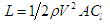 | (2) |
Where, L is lift, ρ is density of air, V is the velocity and Cl is the coefficient of lift.
2.2. Performance Parameters
According to Betz Law a turbine can convert only less than 16/27 (59%) of wind energy to mechanical energy. This law stands for any bare wind turbine. But the research and advances in technology have led to the fact that wind turbines with a shroud can exceed the Betz Limit, as stated by Henson [3]. The experimental study of such shrouded turbines has been carried out by Ghajar and Badr. They experimented with a diffuser-augmented turbine to increase the power output and concluded with an increase in the power augmentation with their design [4]. The power augmentation by using shrouded turbines has been numerically demonstrated by Kannan, Mutasher and Lau. Using CFD, they simulated Diffuser Augmented Wind Turbine to determine the amount of power augmentation with different designs. They concluded with an optimized diffuser design [5]. It is shown that a higher Cp than Betz Limit can be achieved by using a diffuser or shrouded design.The thrust coefficient CT is associated with the thrust experienced by the rotor. It is the ratio of thrust force to the dynamic thrust force. Thrust acts parallel to the turbine axis, so it does not affect the speed of the rotor. For ideal case the value of CT is 8/9. It depends on the loading of the rotor. As stated earlier, it does not affect the turbine's efficiency to convert the available power into electric power. Tip speed ratio λ is defined by the ratio of the speed of blade tip to the speed of the oncoming wind. The selection of this factor is very crucial for the wind turbine design. A high tip speed ratio means the aerodynamic forces are parallel to the axis of the turbine, which implies a high lift to drag (L/D) ratio. When the tip speed ratio is low, it results in lesser aerodynamic efficiency. Due to lower λ, there is a generation of two adverse effects, one is swirl and the other is tip loss. Both these effects are detrimental in the efficiency of the turbine. Keeping in view all these factors, tip speed ratio is chosen.
2.3. Comparison with Low Altitude Turbines
The main difference between high and low altitude turbines is the amount of wind power available. It shown in Figure 1. 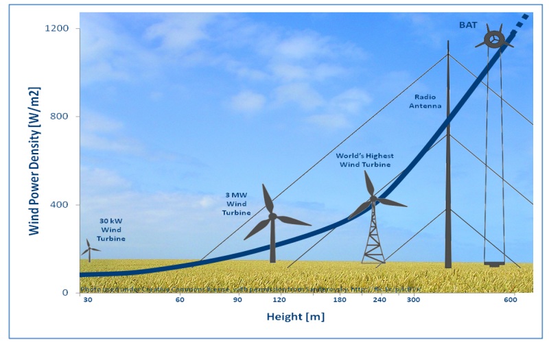 | Figure 1. Power density vs. altitude |
The power density increases logarithmically, as we go beyond the height of conventional wind turbines. The winds are more consistent and uniformly directional at the altitude of above 2000 feet than near the ground. According to the assessment done by Department of Geological and Environmental Sciences, California State University Chico and Department of Global Ecology, Carnegie Institution of Washington, Stanford [6], the jet streams between 7 to 16 km of altitude are much faster than the ones close to the ground. The wind is more uniform in the region above 300 m, due to less disturbances caused by the structures like buildings, towers etc. The turbulence is also very low at higher altitudes. Low altitude turbines have to experience wind shear and heat differences in the wind, due to close proximity to ground. As a result low altitude wind turbines are subjected to fatigue, which results in part failure [7]. As per the FAA regulations, the airborne turbines cannot go beyond a certain height. The wind turbine designed in this paper has the operational height of 100 meters.
2.4. Comparison with Low Altitude Turbines
When a turbine is airborne, a number of loads are expected to act on it. The various parts of the turbine experience different types of loads, so the loads govern the material requirement for each component of the turbine. The main parts for the wind turbine are blades, hub, gearbox, nacelle and a generator. The materials required for the airborne turbine blades need to satisfy the following criteria in order to make it robust, efficient and economic. 1. The materials have to be stiff enough to yield to the optimum aerodynamic performance. 2. The material needs to be light, to reduce the overall weight and the gravity forces. 3. It should be a fatigue life good enough to sustain for a longer time 4. It has to be cheaper to make the model economic. The blades are potential targets for a large number of loads. The blades experience inertial, gravitational, bending, torsional and cyclic loads. There is edgewise bending of the blade caused by gravitational forces and torsional loads. The wind pressure causes the flap wise bending. The root of the blade experiences the highest edgewise bending. They also contribute to the fatigue of the blade determining the age of a blade. The cyclic loads are usually due to the wind turbulence and pressure differences. To withstand all these loads, different parts of the blade are made up of different materials. Strong and light weight composites, matrix and laminates are used in the manufacturing of turbine blades. The nacelle houses the gearbox, generator and other electronic equipment, and protects them from the atmospheric interference. The materials, which are used for the construction of the nacelle, have to be corrosion resistant beside s being strong and light weighted. Glass fiber composites make a good choice for the same.
3. Modeling
3.1. Airfoil Shape Selection
The airflow over the blades of wind turbine behaves exactly similar over an aircraft wing. Therefore, the initial design of the turbine blade is concentrated in choosing the correct airfoil. The following figure describes the important features of an airfoil.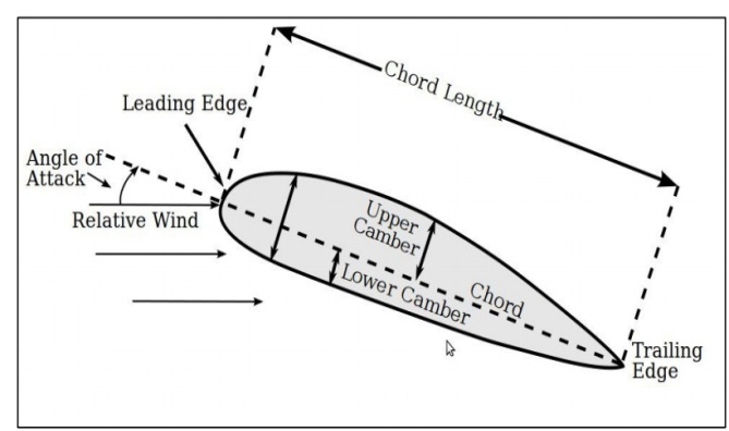 | Figure 2. Airfoil nomenclature [18] |
Leading and trailing edges are the frontal and rear points on the airfoil. The line joining the leading edge to the trailing edge is the chord line. The total length between the leading and the trailing edge is the chord of the airfoil. The camber is distance from the upper and lower surfaces with respect to the chord line. The upper camber is the distance above the chord line and lower camber is the distance below it from the upper and lower surfaces of the airfoil respectively. The distance of the camber is usually measured from the quarter chord point from the leading edge [8].As we know that, it is the pressure difference that develops lift. The lower surface of the airfoil has to be such so that the air flows faster on the top of the airfoil than the lower surface, which means a high pressure at the lower surface and low pressure at the top surface of the airfoil. This phenomenon is also known as the Bernoulli’s principle, as Daniel Bernoulli was the person to show it. This pressure distribution creates a force, which is known as lift. The shape of cambered airfoil is self-sufficient to generate lift, but a certain amount of change of angle with respect to the incoming wind can lead to higher lift generation. This angle is called angle of attack. There is a limit to angle of attack, beyond which the flow separates and the phenomenon called stall occurs. The following figure explains the separation of the flow over an airfoil in detail [9]. The airfoil selection for the turbine has been done by analyzing the NREL (National Renewable Energy Laboratory) airfoils. [10] NREL has data available on various airfoils. The data has been collected by NREL using Eppler Airfoil Design and Analysis Code. The airfoil selected for the turbine here is based on the rotor diameter and the lift of coefficient. Two airfoils have been selected for comparison. S826 and S822 have been analyzed based on the lift characteristics and CL/CD curve. S826 has CL f 1.353 at 60 angle of attack and CL/CD of 139.48 as seen in Figure 4. S822 has CL of 0.911 at 60 angle of attack and CL/CD of 99.02 as seen in Figure 5. Since S826 has higher lift coefficient, it has been selected. For the same reason the primary angle of attack has been chosen as 6° for the blades. The entire blade is made up of the same airfoil for the simplicity. Figure 3 shows the sketch of the airfoil. | Figure 3. Flow behavior over an airfoil |
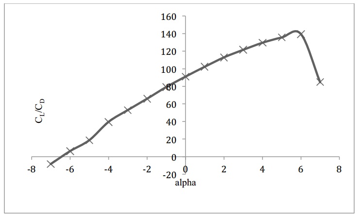 | Figure 4. CL/CD vs. angle of attack for S826 airfoil |
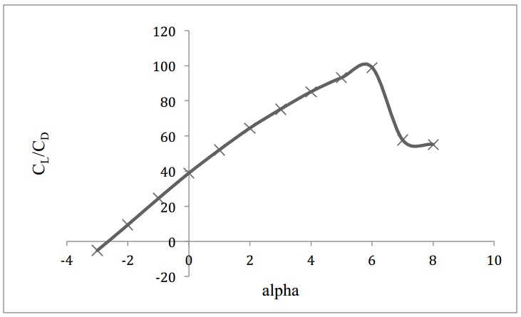 | Figure 5. CL/CD vs. angle of attack for S822 airfoil |
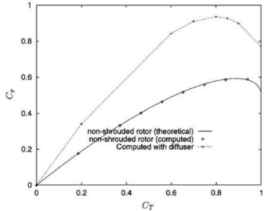 | Figure 6. Efficiency of turbine with shroud and diffuser |
3.2. Dimensioning
The design process started with some initial assumptions. According to Betz limit, the efficiency of a turbine cannot exceed 59%. Most modern wind turbines have efficiency in the range of 20-40% [11], as shown in Figure 6. The aim of the turbine designed in this thesis is to exceed the conventional efficiency limit. Martin Hansen in the second edition of Aerodynamics of Wind Turbines describes the possibility of exceeding the Betz limit by placing the turbine in a diffuser [3]. It has been shown by de Vries in 1979 that the diffuser will increase the mass flow rate through the turbine. The idea is to place the turbine in the diffuser at the throat, as shown in the figure below. The arrow shows the direction of the airflow. Gilbert and Foreman (1983) suggested CFD analysis of turbine with a diffuser, where diffuser was modeled using 266,240 grid points and diffuser airfoil section with 96 points. They used a turbulence model to do the simulation, as it is sensitive to adverse pressure gradients. The results they obtained are depicted in the following figure 6. [3]It can be seen the turbine with the diffuser has achieved Cp of approximately equal to 0.9, which is way too higher than the uncovered turbine Cp of 0.5. So far it has not been applied to a full-scale model, because of the extra structure that might lead to more cost and loads.This paper is focused on the airborne turbine; the balloon that lifts the turbine into the air has been designed in the shape of a convergent divergent nozzle. As a result there are no issues of loads due to extra structure like in the conventional turbines.For the initial designing of the turbine, the efficiency of 80% has been assumed, that is a value of Cp equal to 0.8 and the credibility of this assumption will be seen in the results section. Based on the Cp, the rotor diameter is 7.4m as per the following equation (3)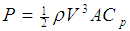 | (3) |
Where, P is power, ρ is the density of the air, V is the velocity of the air at the rotor, A is the area of rotor and Cp is the power coefficient.
3.3. Convergent Divergent Nozzle Shroud
A convergent-divergent type balloon has been chosen to make the turbine go airborne. The use of a ducted structure around turbine helps in increasing the output power of the turbine. It has considerable amount of advantages over bare turbine, which includes reduction of gusts. It eliminates the requirement to have turbine facing the direction of wind all the time, thus yaw mechanism is not needed. It increases the amount of air that passes through the rotor and thus increases the axial velocity and the velocity of the air on the blades. The reason behind this being that when the turbine is placed at the throat of convergent divergent nozzle, low pressure is induced near the throat which tends to draw more amount of air into the rotor. More the mass flow rate through the rotor more is the energy produced. The concept revolves around increasing the energy density of air [12].
3.4. Formulation
This section describes step by step, how the turbine has been designed. The turbine has 3 blade configuration, the tip speed ratio λ = 7.5 and the blade is buildup of NREL S826 airfoil with CL = 1.434 at 6° angle of attack. The following describe the formulation of all the design features of the turbine as shown in Figure 7.1. Rotor Radius, R: As the required power from turbine is 70kW, CP is chosen to be 0.8 and the velocity of air is 10m/s, from the following equations the radius of the rotor and length of blade are calculated.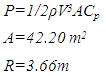 The radius of hub has been selected as 0.25m, thus the length of blade is l = 3.41m.
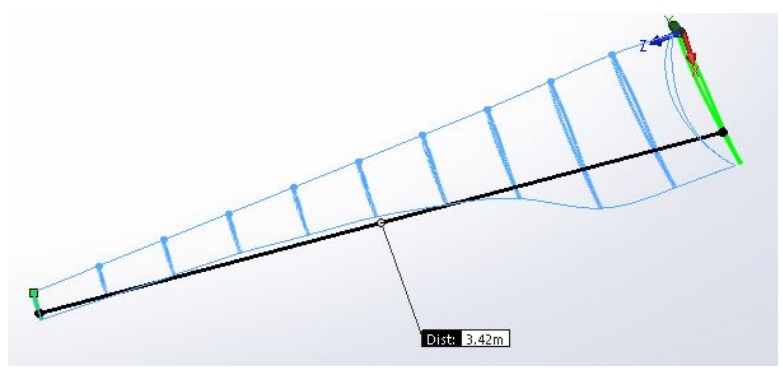 | Figure 7. Turbine blade |
2. Rotational Speed, n: The following relations describe the rotations done by a blade in one second.n = V/2ΠR = 0.959 s-13. Angular Speed, Ω: It is given by the following relation Ω = n2Π = 6.02 rad/s4. Tip Speed, VT: The speed at the tip of the blade is given asVT = XV = 75 m/sThe length of the blade has been divided into 10 equal sections and the various characteristics have been calculated as per given in the table below.Table 1. Design Features of Turbine
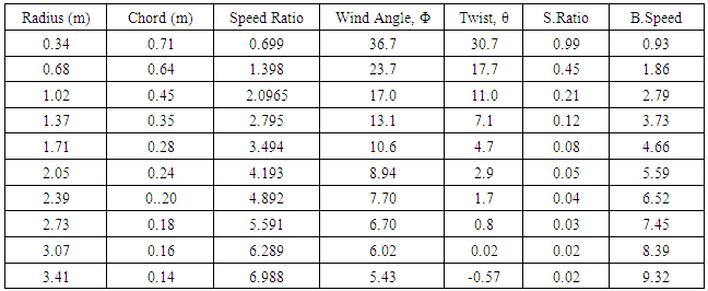 |
| |
|
The shroud around the balloon is in a convergent-divergent shape. The ratio of inlet area to throat area, Ai/At = 1.31 and exit area to throat area, Ae/At = 1.15. The turbine is positioned at the throat of the converging-diverging shaped balloon. The length to throat diameter ratio, LS/Ds = 0.8. The contraction angle is 20°. The area ratios have been selected after doing extensive literature review [4], [5], [13], [14].
3.5. Estimation of Weight and Volume of Turbine
From the SolidWorks model as shown in Figure 8&9, the weight of the rotor is estimated around 380 kg. In case of conventional wind turbines the weight of the rotor is around 13% of the entire machine. The weight of machine is estimated asW Machine = W Rotor / 0.13W Machine = 2923 kgOut of this 2923 kg, 60% of weight is for the tower that supports the conventional wind turbine. So, in case of the airborne wind turbine this weight is neglected. Thus, the actual weight of machine is estimated asWActual_Machine = 2923 – 1753 = 1169 kgArchimedes Principle states that the buoyant force on a submerged object is equal to the weight of the fluid that is displaced by the object. The same principle is applied when the turbine is made airborne with the help of shroud around it.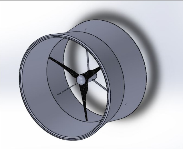 | Figure 8. Isometric view of turbine |
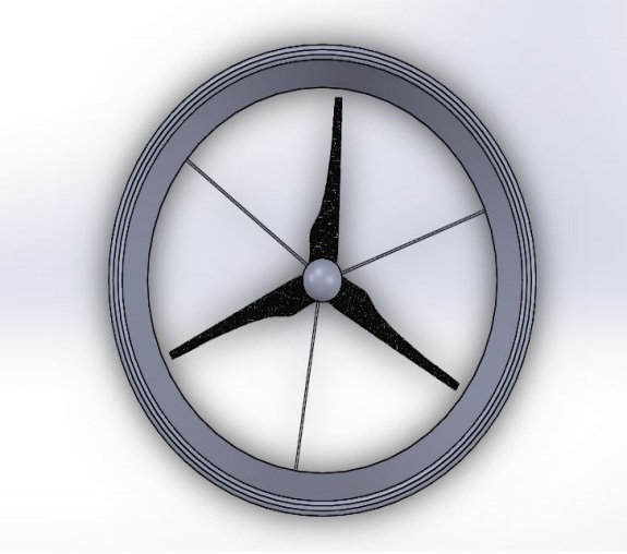 | Figure 9. Front view of turbine |
Mass lifted or Payload = Mass of the fluid displaced Hence, the volume of air displaced is equal to volume of the shroud.V Shroud = 1169/1.2 = 974.17 m3Hence, mass of turbine required is, M T = 974.17 * 0.18 = 175.35 kg, where 0.18 is the density of turbine in kg/ m3. The mass of shroud that can hold 974.17 m3 of air is calculated around 110 kg. The material used for shroud is same as used by the air balloons, which is Dacron with a density of 1380 kg/m3.
4. CFD Analysis
Computational Fluid Dynamics has been used to analyze the performance of the turbine. The analysis has been performed using Star CCM+ 9.02 software, which is owned by CD-Adapco. Star CCM+ is capable of performing calculations based on the model properties that are chosen for any particular analysis. The algorithms in the model solves for numerous outputs based on the inputs given to it. In the analysis, the air works like an ideal gas, thus the model uses the ideal gas equation ρ = P/RT, where ρ is the density of the air at the operating altitude of the turbine, P is the absolute pressure, R is the gas constant and T is the temperature. The model operates at sub-sonic conditions. The model uses Navier-Stokes equation and momentum equation. The turbulence model used for analysis is K-ε (K-Epsilon). This model has been chosen keeping in consideration the application, physics involved and the capability of the computer available. K-ε is a robust model, which is simple and the most common in industrial applications. This model emphasizes on the two terms K, which represents the turbulent kinetic energy and ε, which represents the dissipation rate [15].The model of the turbine and shroud around it were drafted using SolidWorks. It was meshed using Star CCM+. The Unsteady Reynolds Averaged Navier Stokes Simulation (URANS) with K-ε turbulence model has been used to study the flow properties around the turbine blades and the performance of the turbine. The physical time for the simulation is 20 seconds, with the time step of 0.005 seconds. The flow has been divided into two regions. The first one represents the flow in the turbine region and the second region represents the flow that is going into and coming out of the shroud. Each region is an interface to allow for rotation of wind turbine and hub. The other method of analyzing moving part in a fluid is using the technique called over set mesh, but that is more complex in nature and has to perform numerous iterations compared to the technique used here.The meshing has been done using Star CCM+, with a refinement around rotor blades and the hub. The percentage of base is 1 and absolute size is 0.01m. The number of prism layers is 2. The mesh configuration for the two regions is given in the table below:Table 2. Meshing Features
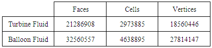 |
| |
|
The physical conditions include the flow direction, which is Boundary-Normal; for Free Stream Option Mach Number, Pressure and Temperature have been selected. The Mach Numbers are 0.035 and 0.020, Static Temperature is 278.15 K, Turbulence Intensity is 0.01 and Turbulence Viscosity Ratio is 10. The Shear Stress Specification is no-slip condition. Tangential Velocity Specification is relative to mesh. Figure 10 shows the Meshed model in CFD. Thermal specification is adiabatic. Wall surface has been selected as smooth. The physical values for epsilon and kappa are 9.0 and 0.42 respectively. The velocity of air is 12 m/s and 6 m/s, for Run 1 and Run 2, respectively. For initial conditions, the continuum values have been selected. The motion of this region is static [16].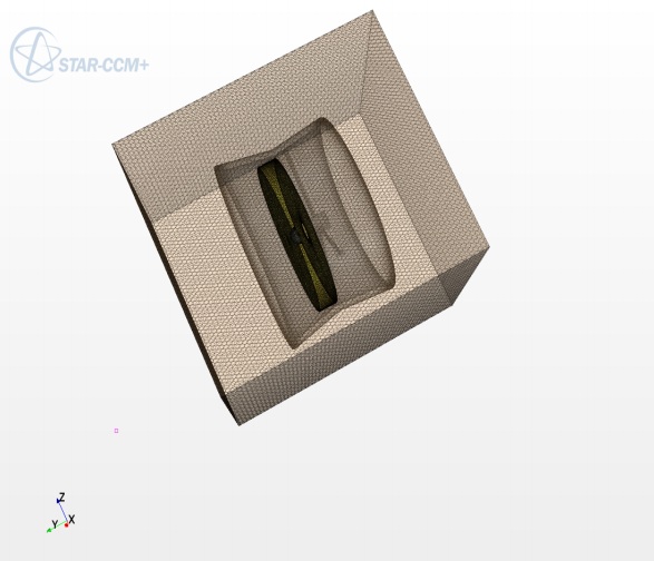 | Figure 10. Meshed model in CFD |
5. Results and Discussion
Two Star CCM+ simulations have been performed with 12m/s as the ambient velocity in first run and 6m/s in the second run. The torque of the turbine has been recorded at 739 N-m for Run 1. The velocity profile of the blade has also been analyzed which varies from 0.036 m/s to 111.12 m/s for Run 1, from root to the tip of the blade. The velocity and pressure profiles have been recorded at every iteration.Run 1: Figure 11 shows the velocity of the blade from root to tip. It varies from 0.036 m/s at the root to 111.12 m/s at the tip. The theoretical value of the tip velocity is 75m/s. From the CFD results the average tip velocity is 79 m/s.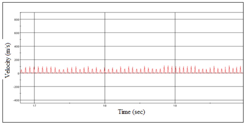 | Figure 11. Blade velocity vs. time |
Thus, the chosen tip speed ratio of 7.5 has been verified. The tip speed ratio is an important factor in the efficiency of a wind turbine. If the blades move too fast then they will act as a wall to the incoming air, thus there will be low lift generation. If the blades move slowly, then the air will pass through the gaps of the blades. The speed of blade from root to tip from the simulation confirms that the blades are moving with a reasonable speed. Figure 12 shows, the increase in torque with time and achieves a constant value of around 750 N-m. During the entire simulation, the turbine is spinning free. The torque seeks a constant value after a certain period of time. The amount of torque generated depends on the angular velocity. If the angular velocity is high, higher torque generation results in higher power. From Figure 12, it is clear that the turbine is gaining a constant torque. After 11.5 sec, the airflow is stabilizing and torque value is gaining steady value.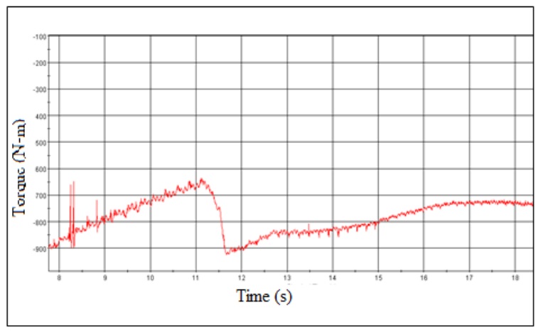 | Figure 12. Torque vs. time |
Figure 13 shows the rotation of the rotor blades, as the position of the blades changes. From these contours the velocity of the blade from root to tip can be seen varying as per obtained from the velocity plot. It increases from root to tip of the blade.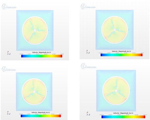 | Figure 13. Blade velocity contours |
The color contour exhibits the tip velocity is around 70-80 m/s. The position of blades at different instants has been shown in this figure. The rotation of turbine is evident, thus confirms that the blades are rotating and generating lift. The tip velocity matches with the theoretical value to a huge extent. The tip speed obtained from numerical analysis is larger by 5% than the theoretical value. Figure 14 shows the scalar midplane velocity. The turbine is inside the shroud and the contours show the behavior of air entering the shroud. The increase in velocity of the air from the point of entering the shroud to the throat, where the air interacts with the rotor plane, can be seen very vividly. From these contours, the air is getting more streamlined before it hits the rotor plane. The inlet of the shroud is providing a better flow direction to the incoming air. A low velocity can be observed in few regions like behind the nacelle, at the shroud edges facing the airflow.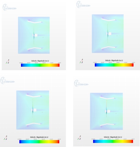 | Figure 14. Scalar midplane velocity |
Figure 15 shows the velocity vector contours. The rotation of the turbine can be seen around in the midplane. The velocity of the air can be seen increasing inside the shroud, near the rotor. These contours provide the value of the velocity at the throat of the shroud. Hence it provides the power available at the throat and the amount of power available for conversion to mechanical power by the turbine. The average velocity of the air is 16 m/s in the plane of rotation. From these contours the velocity vectors can be seen getting better directed towards the rotor. This also supports the fact that air entering the shroud is more streamlined, as explained by Figure 16.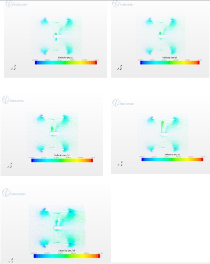 | Figure 15. Blade velocity contours |
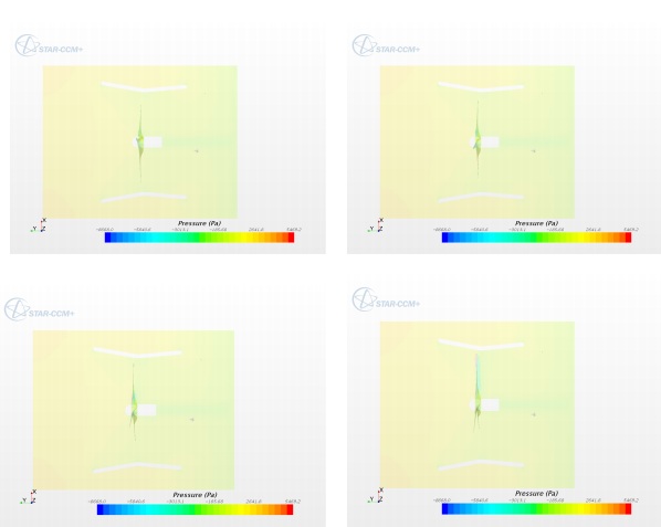 | Figure 16. Pressure contours |
Figure 16 shows the pressure distribution inside the shroud. The pressure on the blades can be seen changing from high to low on lower surface to upper surface respectively. This explains the fact that the blades are generating lift.Run 2: For Run 2, the ambient velocity chosen is 6 m/s. Vector midplane velocity and blade velocity contours have been studied. The scalar midplane velocity and pressure contours exhibit similar trend as the Run 1.From blade speed contours, the average tip velocity is 58 m/s. So, at 6 m/s velocity the blade speed is not as much as achieved at 12 m/s ambient velocity.Figure 17 shows the velocity of the air that enters the shroud. The velocity of the ambient air is 6 m/s, so the average velocity achieved at the throat is approximately around 10 m/s. The flow behaves in the similar way as in Run 1. The velocity achieved at the throat region of shroud is 16 m/s for Run 1 and 10 m/s for Run 2, respectively.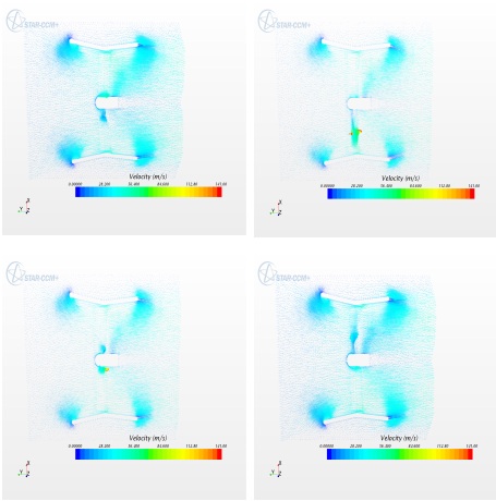 | Figure 17. Vector midplane velocity for run 2 |
The velocity achieved at the throat region of the shroud is 16 m/s for Run 1 and 10 m/s for Run 2, respectively. So the power of the wind has been calculated as PW = ½ ρV3A = 103 kW for Run 1 and Run 2 is 25 kW. The value of axial force coefficient chosen is 0.33, because that is where the maximum power is produced. The actual power produced by the turbine is given by the following PT = 2ρV3Aa (1-a) 2 = 61 kW for Run 1 and 14 kW for Run 2, where a is axial induction factor. It can be seen that for Run 2, the power generated is too low as per the requirements. The coefficient of power CP is obtained by the following relation.CP = PT / PW = 0.59so, the efficiency of the current turbine and shroud is 59%, which is higher than any fixed wind turbines, but not to the extent as projected. Figure 18 shows the variation of power with respect to a. After an equals 0.33, the power goes down. This plot shows the power curves for two different ambient velocities.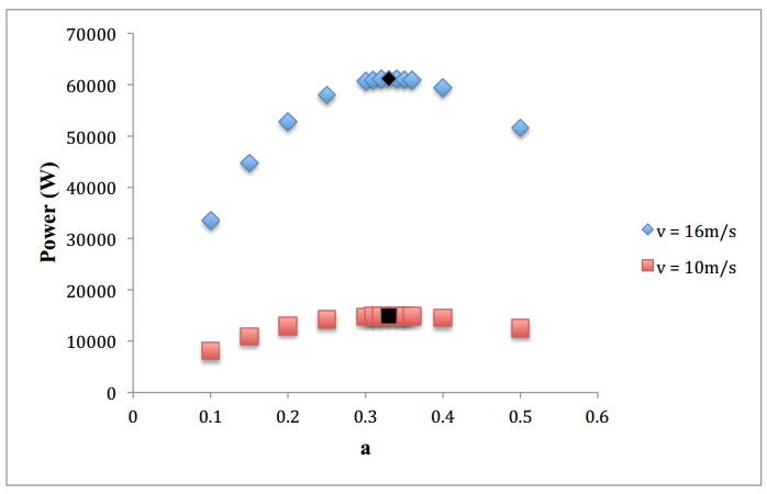 | Figure 18. Power vs. a curve |
Figure 19 shows the variation of power as the velocity increases. The point highlighted shows the operational speed of the turbine and the power generated by it.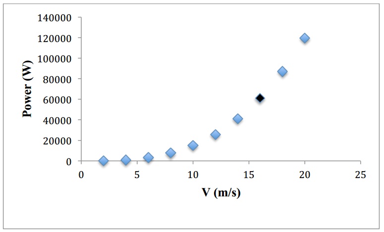 | Figure 19. Power vs. velocity curve |
6. Conclusions
The full-scale model of the shrouded wind turbine has been analyzed using CFD software StarCCM+. The theoretical and numerical data have been compared. The theoretical and numerical values match considerably. The turbine blades have been designed using the BEM modeling. The airfoil used for blades is NREL S826 and the entire blade is buildup of the same airfoil. The rotor diameter is 7.4 m. The shroud around the turbine has been designed as a convergent-divergent nozzle shaped balloon. The ratio of inlet area to throat area, Ai/At = 1.31 and exit area to throat area, Ae/At =1.15. The turbine is positioned at the throat of the converging-diverging shaped balloon. The length to throat diameter ratio, LS/DS = 0.8.For Run 1, the velocity of air near the rotor was expected to increase from 12 m/s to 15 m/s theoretically; while from CFD analysis velocity recorded was 16 m/s. The increase in velocity was achieved by the convergent-divergent shaped shroud around the turbine. The convergent-divergent nozzle increases the mass flow rate through the turbine by increasing the velocity thus producing higher power than a bare turbine. With the velocity of 16 m/s, the value of CP calculated is 0.59, thus power produced the velocity of 16 m/s, the value of CP calculated is 0.59, thus power produced is 61 kW.The amount of power that was expected from this design was 70 kW, based on the assumption that CP value was 0.8.For Run 2, the velocity was 6 m/s and it increased to 10 m/s near the throat, but could only generate 25 kW of power. From the analysis, it can be concluded that velocity of the air hitting the rotor has to be more than 20 m/s to produce higher power. The higher velocity can be achieved by changing the shape of the throat around the turbine. Due to the presence of shroud around the turbine the airflow follows a smooth direction towards the rotor, which is absent in bare wind turbines. This observation is important from the fact that, yaw mechanism is not required in such a favorable situation. The concept of shrouded airborne turbine is economical and environment friendly. The emission of carbon dioxide and other gases like nitrogen oxide by the boats in current use will be completely eliminated. This concept can be applied to produce energy for ships. Besides, airborne wind turbine can be used to produce electricity for houses, buildings, etc. From the entire analysis, the concept presented in this paper is promising for future consideration. It has the capability of addressing the issues of energy crisis and environmental issues that the humankind is facing now and is going to face in coming years.
References
| [1] | U.S. Energy Information Agency, 2015 “What is U.S Electricity Generation by Energy Source,” http://www.eia.gov/tools/faqs/faq.cfm?id=427&t=3. |
| [2] | Leisurecat, 2015 “Range of Models,”http://www.leisurecat.com.au/our-boats/range-of-models/leisurecat-350-sports-express/. |
| [3] | Hansen, M. O. L., 2008 Aerodynamics of Wind Turbines, 2nd edition, Earth scan New York 52. |
| [4] | Ghajar, R. F., and Badr, E. A., 2008 “An Experimental Study of a Collector and Diffuser System on Small Demonstration Wind Turbine,” International Journal of Mechanical Engineering Education, 36(1), pp. 58-68. |
| [5] | Kannan. T. S., Mutasher, S. A., and Lau, Y. H. K., 2013 “Design and Flow Velocity Simulation of Diffuser Augmented Wind Turbine,” Journal of Engineering Science and Technology, 8(4), pp. 372-384. |
| [6] | Archer, C. L., and Caldeira, K., 2009 “Global Assessment of High-Altitude Wind Power,”. |
| [7] | Wind Power Engineering, 2015 “How Turbulent Winds Abuse Wind Turbine Drivetrains,”http://www.windpowerengineering.com/design/how-turbulentwind-abuse-wind-turbine-drivetrains/. |
| [8] | Shields, M., and Mohseni, K., "Static Aerodynamic Loading and Stability Considerations for a Micro Aerial Vehicle," paper presented at American Institute of Aeronautics and Astronautics Applied Aerodynamics Conference, Chicago, IL, 28 June - 1 July 2010. |
| [9] | NASA, 2015 “Work of Wings,”http://virtualskies.arc.nasa.gov/aeronautics/3.html. |
| [10] | NREL, 2009 “Index Of /Airfoils/Coefficients,”http://wind.nrel.gov/airfoils. |
| [11] | Perso Bertrand Blanc, 2015 “Wind Turbines Efficiency & Comparison Calculator,”http://perso.bertrand-blanc.com/Resume/Experience/Enery/. |
| [12] | Wind Energie, 2015 “Concentrating Wind systems - Sense or Nonsense?”http://www.heiner-doerner-windenergie.de/diffuser.html. |
| [13] | Chris, K., Filush, A., Kasprzak, P., and Mokhar, W., 2012 “A CFD Study of Wind Turbine Aerodynamics,” ASME. |
| [14] | Amano, R. S., and Malloy, R. J., 2009 “CFD Analysis on Aerodynamic Design Optimization of Wind Turbine Rotor Blades,” World Academy of Science, Engineering and Technology, 3, pp. 12-14. |
| [15] | Schroeder, E. J., 2005, "Low Reynolds Number Flow Validation using Computational Fluid Dynamics with Application to Micro-Air Vehicles," master's thesis, University of Maryland, College Park. |
| [16] | Khalid, M., August 1988, "Use of Rib lets to Obtain Drag Reduction on Airfoils at High Reynolds Number Flows," Scientific and Technical Publications, NRC 29459, National Research Council Canada. |

 Abstract
 Reference
 Full-Text PDF
 Full-text HTML