Swapnil Pramod Kanade, Abraham T Mathew
Department of Electrical Engineering, National Institute of Technology, Calicut, 673601, Kerala
Correspondence to: Swapnil Pramod Kanade, Department of Electrical Engineering, National Institute of Technology, Calicut, 673601, Kerala.
| Email: |  |
Copyright © 2012 Scientific & Academic Publishing. All Rights Reserved.
Abstract
Robustness is the ability of a control system to maintain its performance and stability characteristics in the presence of all uncertainties. Attitude control of rocket is a benchmark problem in aerospace and missile guidance control because such a system is subjected to number of uncertainties like flight path change, mass variation, thrust variation, drag and so on. In this paper the robust control techniques for attitude control of rocket has been examined. The control problem consists of actuating of fin deflections by the autopilot which modifies angle of attack and sideslip angle while stabilizing the rocket rotational motion. In order to separate the uncertainties from nominal model, the uncertainties are expressed as diagonal structure in form of ULFT (Upper Linear Fractional Transforms) which avoids unnecessary conservation. Then 2 DOF H-∞ loop shaping technique is carried out for pitch rate control problem. This has been compared with H-∞ controller design technique. It has been observed that 2 DOF H-∞ loop shaping technique can provides good robust stability and performance. Extensive simulations have been carried out to evaluate system performance. The comparative results are included in this paper.
Keywords:
Robust Control, H-∞ Loop Shaping Control, Robust Performance
Cite this paper: Swapnil Pramod Kanade, Abraham T Mathew, 2 DOF H- Infinity Loop Shaping Robust Control for Rocket Attitude Stabilization, International Journal of Aerospace Sciences, Vol. 2 No. 3, 2013, pp. 71-91. doi: 10.5923/j.aerospace.20130203.02.
1. Introduction
Rockets differ from aircraft and spacecraft due to the rapidly time-varying parameters of their equations of motion, which often requires special guidance and control design strategies and short duration of flights. Furthermore, the fast response times required in both translation and rotation of rockets necessitate a much larger control loop bandwidth than that of either an aircraft or a spacecraft.With the advancement in control theory, it is now possible to design control system using MIMO frame work. Also are new mathematical approaches that take into account for the modeling uncertainties, disturbance & measurement noise and render a robust controller. New methods have appeared in literature for attitude control of rocket. Forexample optimal control adaptive control , nuero- fuzzy control, robust control lyapunov based control design and genetic algorithm development. Adaptive technique assures high computation speed.The rocket should be able to perform some maneuvers. This may include larger angle of attack, rapid rotational rate change, larger angular acceleration and wide variation in pressure and speed. This makes control problem challenging that requires guaranteeing robust stability and robust performance in presence of large parameter variationandunmodelled dynamics with nonlinearities. In 1981 Zames[1] brought H-∞ norm as a performance requirement. H-∞ control techniques developed by Doyle et al[2] ,Glover et al[3] not only offers the tradeoff between performance and control effort but also provides thecapabilities of accommodating the disturbance and parametervariation. Reichert[4] was the first to apply H-∞ control and to show how it advantages over classical control in autopilot design. Similar autopilot designs were considered byReichert Wise and Jackson. The autopilot robustness uncertain aerodynamic parameters are also examined by Wise. From[11] we see that the H-∞ loop shaping controller was proposed by McFarlane and Glover in 1990. The systematic procedure was developed by Hyde in 1993. After that Limbeer,Kasenally and Perkinns extended it to 2 DOF loop shaping controller development and formulate standard H∞ optimization problem which allows to use model matching function in robust stabilization. In this paper 2 DOF feedback H-∞ loop shapingtechniques is applied for pitch rate control of rocket. Application to rocket model shows that closed loop system for pitch rate control is robust under structural natural frequency variation. In this paper aerodynamic data which is the function of Mach number 2.78 used for design purpose and the parameters are related to that described in[8]. The controller shouldguarantee stability for the model in addition to the performance specification that will be demanded.Remaining part of the paper is organized as follows.Section 2 describes about system modeling and equations ofmotion, linearization of model, uncertainty modeling. Section 3 includes 2 DOF loop shaping design details. Section 4 contains results, discussion & limitations of two approaches. Section 5 describes conclusion.
2. System Modeling
The model of rocket is first derived using 6 DOF custom variable mass blocks.The six degrees of freedom consist of three translations, and three rotations, along and about the missile ( Xb ,Yb, Zb ) axes. These motions are illustrated in Figure (1) the translations being (u,v,w) and rotation (P,Q,R) . Following Figure 1 shows complete 6 DOF representation of rocket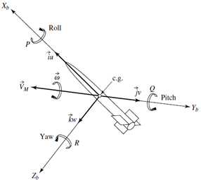 | Figure 1. 6 DOF representation of rocket |
In compact form, the translation and rotation of a rigid body may be expressed mathematically by the following equations.Translation: ∑ F=maRotation: 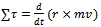
2.1. Assumptions for Modeling of Rocket & Rocket Model Analysis
No model can be truly depicting its real system. So the model is only approximate representation of the behavior of the real system. The model for the rocket is derived based on following assumptions:[6],[9]1. The rocket equations of motion are written in the body-axes coordinate frame.2. A spherical Earth rotating at a constant angular velocity is assumed.3. The vehicle aerodynamics are nonlinear.4. The winds are defined with respect to the Earth.5. An inverse-square gravitational law is used for the spherical Earth model.6. The gradients of the low-frequency winds are small enough to be neglected.7. A constant mass will be assumed, that is dm/dt =08. The aerodynamic forces and moments acting on the vehicle is assumed to be invariant with the position of rocket relative to the free stream velocity vector. Consequently the assumption greatly simplifies the equation of motion by eliminating the aerodynamic cross coupling terms between roll motion and pitch, yaw motion. In addition a different set of aerodynamic characteristics for pitch and yaw is not required. | Figure 2. Pitch plane force diagram |
In controller design only pitch perturbation motion is considered. In this case rocket attitude is characterized by pitch angle θ and flight path angle Θ or equivalently angle of attack α and θ. Due to rocket symmetry the yaw stabilization system is analogous to pitch stabilization system[7] . Hence equation of motion in pitch plane is considered. Thefollowing Figure 2 shows complete free body diagram for pitch plane analysis with mathematical equations.[8-10].In following Figure 2 reference frame notations used for writing equations of motion as the x* -axis of thevehicle-carried vertical reference frame is directed to the North, the y* -axis to the East. The x1-axis of the body-fixed reference frame is directed towards to the nose of the rocket, the y1- axis points to the top wing. The x-axis of the flight-path reference frame is aligned with the velocity vector V of the rocket and the y-axis lies in the plane x1 y1.1. Equations describing the motion of the mass centre | (1) |
 | (2) |
whereP = engine thrust.Q = aerodynamic drag. generalized disturbance forces in x, y direction.m = mass of rocket V = velocity of rocket2. Equations, describing the rotational motion about the mass centre
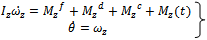 | (3) |
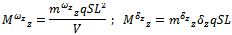
wher  the rocket moments due to the angle of attack α
 the aerodynamic moments due to pitch rate ωz
 the control moments due to fins deflection δz
 generalized disturbance moments about corresponding axes.
 pitch rate change3 Equation giving the relationships between the angles α, θ, Θ
  | (4) |
4 Equation giving the normal acceleration 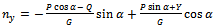 | (5) |
2.2. Linearization of Equations
In order to obtained a linear controller equations (1) – (5) are linearised about trim operating points
 under the assumptions that the variations

 are sufficiently small. In such a case it is fulfilled that sinΔα ≈ Δα, cos α ≈ 1.As a result, the linearised equations of the perturbed motion of the rocket take the form
 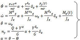 | (6) |
where
 equations (6) can be represented as
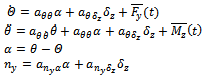 | (7) |
where 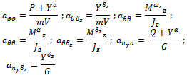 In (7) we used the notation
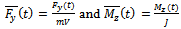 Equations (7) are extended by the equation describing the rotation of the fins
 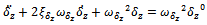 | (8) |
Where  is the desired angle of fins deflection (the servo actuator reference);
  is the natural frequency and
  is the damping coefficient of servo actuator. The set of equations (7) and (8) describes the perturbed rocketlongitudinal motion. The coefficients in the motion equations are to be determined for the nominal (unperturbed) rocket motion. Nominal values of the parameters are assumed in the absence of disturbance forces and moments.The unperturbed longitudinal motion is described by the equations .
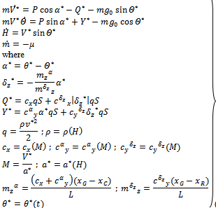 | (9) |
In these equations,  is the desired time program for changing the pitch angle of the vehicle.
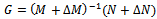
2.3. Nominal Model and Stability of Model
A nominal system model has been obtained using the parameters given in the Table 1. The model is described in form of 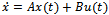
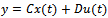 Here
Here  is the input vector
  is the output vector.
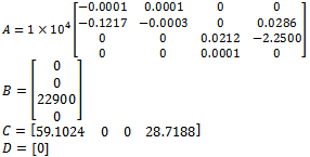 For matrix A, the Eigen values
  corresponds to stable mode and this pair explains system slow dynamics behavior. The pair
  gives the unstable mode and explains about system fast dynamics. Controllability index is 4. And hence system is fullycontrollable. The observability index is 4 and hence system is fully observable. It is require to design
  given by
  This will give a robust performance.
Table 1. System parameters
 |
| |
|
2.4. Uncertainty Modeling
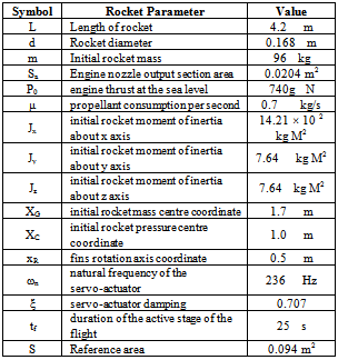
Separation of different uncertain parameters in different parts of model and combining into one block and forming ULFT is basic principle of uncertainty modeling[12]. For above rocket model main variation of coefficients ofperturbed motion happens in aerodynamic coefficients  and these are the function of mach number[7]. For above model 7 coefficients are considered as uncertainty given in equation (7). The uncertainty block △ of all coefficients of variation is diagonal matrix of size 7×7. Complete ULFT model is shown in Figure 3
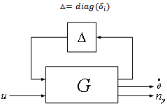 | Figure 3. ULFT representation of model |
3. H-∞ Loop Shaping Design
The loop-shaping design procedure described is based on H ∞ robust stabilization combined with classical loopshaping, as proposed by McFarlane and Glover 1992[5]. The open-loop plant is augmented by pre andpost-compensators to give a desired shape to the singular values of the open-loop frequency response. Then the resulting shaped plant is robustly stabilized with respect to co prime factor uncertainty using H-∞ optimization. The H-∞ can make a balance between robustness, performance and stability of closed loop system .
3.1. Robust Stabilization Against Normalized Coprime Factor Perturbations[11]
To the normal system G constitutes left coprime factorization . Considering its uncertainty a perturbed model as shown in Figure 4 can be described by
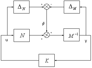 | Figure 4. Normalized coprime factor uncertainty description |
 | (10) |
where  are unknown but stable transfer functions that represent uncertainty in nominal plant model. The design objective of robust control is to make normal model G and family of perturbed plant stable. The family of perturbed plant is defined by
 | (11) |
where  is stability margin. Using small gain theorem the feedback system is robustly stable if (G,K) is internally stable and
 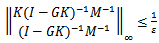 | (12) |
In order to maximize the stability margin it needed to minimize the 
 | (13) |
Here  is the H-∞ norm from ϕ to
 is the sensitivity function for this positive feedback arrangement. The lowest achievable value of
  and corresponding stability margin
  are given as
  | (14) |
where  denotes the Hankel norm of system
  denotes the spectral radius, and for minimal state space realization of G , Z is unique positive definite solution to algebraic Riccati equation
  | (15) |
where  X is unique positive definite solution to algebraic Riccati equation
  | (16) |
A controller which guarantees that 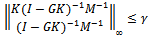 for specified
  is given by
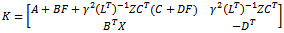 | (17) |
where | (18) |
 | (19) |
3.2. Two Degree of Freedom Controllers[10],[11]
In Doyle et al. and Limebeer et al.[5] a twodegrees-of-freedom extension of the Glover-McFarlane procedure was proposed to enhance the model matching properties of the closed-loop . With this the feedback part of the controller is designed to meet robust stability and disturbance rejection requirements in a manner similar to the onedegree-of-freedom loop-shaping design procedure except that only apre-compensator weight W is used. It is assumed that the measured outputs and the outputs to be controlled are the samealthough this assumption can be removed as shown later. An additional pre filter part of the controller is then introduced to force the response of the closed-loop system to follow that of a specified model M called as reference model.
3.2.1. Scheme of 2 DOF Control
2 DOF H∞ loop shaping control is a robust controltechnique where the time domain specification can be incorporated in the design. The controllers designed by this approach are feed-forward pre-filter and feed- back controllers. The feed - forward pre-filter controller (K1)is adopted to control the time domain response of the closed loop system, and the feed-back controller is designed for achieving the desired robust stability and the disturbance rejection requirement [10]. In this technique, only a pre compensator weightfunction (W1) and reference model (Mref) is needed to be specified. The shaped plant (Gs) is formulated as the normalized co prime factor which separates the nominal plant into normalized nominator & denominator (Ns,Ms) respectively.The design problem is to find out stabilizing controller  with normalized coprime factorization
  which minimizes the H∞ norm of the transfer function between the signals
  as defined in Figure 5. Here
  is a scalar value specified by the designer to assign the degree of significance of the time domain specification.The control signal
  to the shaped plant is given by
  | (20) |
where K1 is a pre filter and K2 is a feedback controller , β is scaled reference and y is measured output. The purpose of pre filter is to ensure that  | (21) |
From Figure 5 we have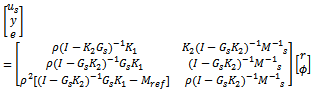 | (22) |
Here  is a scalar value specified by the designer to assign the degree of significance of the time domain specification[11].
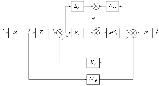 | Figure 5. 2 DOF H-∞ loop shaping design |
To put the 2 DOF design problem into the standard control configuration, we can define a generalized plant P by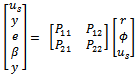 | (23) |
 | (24) |
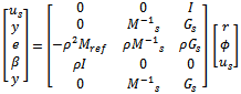
Further if the shaped plant Gs and desired stable closed loop transfer function Mref have the following state space realizations. | (25) |
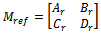 | (26) |
Then P may be realized by 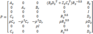 | (27) |
And used in standard H ∞ algorithm to synthesize controller K. note that Rs and Zs are the unique positive definite solution to the generalized Riccati equation (15).
3.3. Design Procedure
The procedure to design 2 DOF H-∞ loop shaping controller as follows[11]:1. Specify the pre-compensator weighting function (W1) for achieving the desired open loop shape.2. Specify Mref which is the desired closed loop transfer function for time domain specifications and select 𝜌 which is a scalar value between 0 and 1. If the designer selects  = 0, the 2DOF H-∞ loop shaping control becomes the 1DOF H-∞ loop shaping control.3. Find optimal stability margin
  by solving following equation
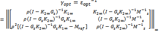 4. Select the stability margin and then synthesize controllers (K1∞,K2∞) that satisfy
 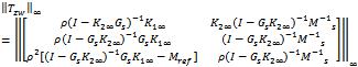 The elements (1,1) and (2,1) help to limit actuator usage, elements (2,2) and (1,2) are associated with robust stability optimization, (3,1) is used to model matching and element (3,2) is linked to the robust performance of the loop.5. Wi is a scalar vector which is given by
 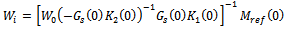 Where
Where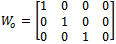 6. Final the feed forward pre filter and feedback controller (K1 and K2) can be determined by following equation
 The schematic diagram of controller is given in following Figure 6.
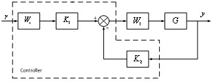 | Figure 6. 2 DOF H-∞ loop shaping controller diagram |
4. Simulation Results and Comparison of H-∞ Controller and H-∞ Loop Shaping Controller Design and Analysis
4.1. H-∞ Controller Design and Analysis
In our study the rocket parameters are selected from Table 1. Figure 7 shows generalized structure of H-∞ controller[13].To design H-∞ controller, select the weight functions in such way that controller order will be equal to total number of system states plus weight function[14]. Basic requirement of weight function is to tune the controller[14].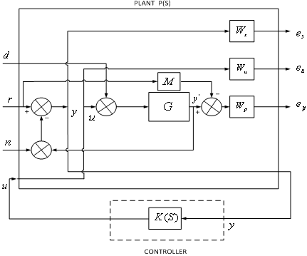 | Figure 7. H-∞ generalized feedback control system |
 | Figure 8. Nominal performance for H-∞ controller |
The sensitivity weight function is selected as 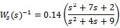 Similarly complimentary sensitivity function is selected as
  The tracking performance weight function Ws is aimed at minimizing low frequency tracking error and the robustness weighting function Wp is to reject high frequency multiplicative uncertainties[14]. In addition the control energy weight function is selected as
  The objective is to avoid actuator operating at high frequencies which lead to saturation[16] . The model matching function is the ideal model to be matched by designed closed loop system which can be selected as[16]
 The actuator noise weight function chosen as
 With above data H-∞ controller is designed. The γ value obtained is 0.1509 which satisfies small gain theorem[12]. The nominal performance is analyzed and it is 0.00039808 as shown in Figure 8. The frequency response of structured singular values for the case of robust stability is shown in Figure 9. The maximum value of μ is 0.47663 which means that stability of closed loop system is preserved under all perturbations that satisfy
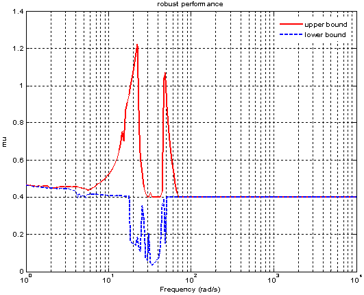
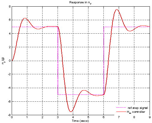
  [12] .The frequency response of μ for the case of robust performance analysis is given in Figure 10. The peak value of μ is 1.22245 which shows that robust performance has not been achieved. Figure 11 shows the transient response of closed loop system with designed H-∞ controller for step signal with magnitude
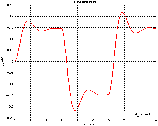
  which corresponds to change in normal acceleration. The overshoot is 22.74% and settling time is 2.84 sec. The fins deflection obtained is 0.1881 rad. ( 11.78°) as shown in Figure 12. The pitch rate variation obtained is 0.1232 (rad/sec) shown in Figure 13 .
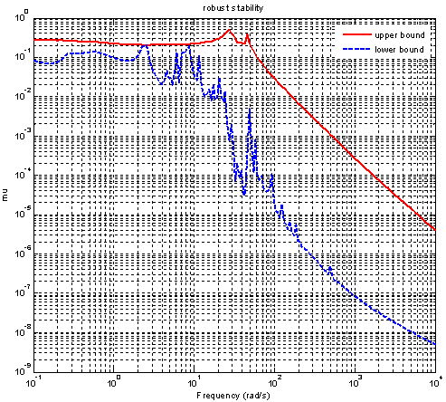 | Figure 9. μ- Robust stability for H-∞ controller |
 | Figure 10. Robust performance for H-∞ controller |
 | Figure 11. Acceleration response for H-∞ controller |
 | Figure 12. Fins deflection response for H-∞ controller |
 | Figure 13. Pitch rate response for H-∞ controller |
4.2. H-∞ Loop Shaping Controller Design and Analysis
Here in attitude controller of rocket is designed with  and pitch rate as feedback inputs. The pre compensator W1 selected as
 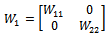 where
where 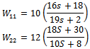 Pre compensator is always a PI form to have enough slope in the cross frequency while low gain in high frequency can provide enough damping to gain the robustness[17]. The post compensator W2 is selected as
  where
where 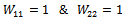 Post compensator generally reflects the relativeimportance of outputs to be controlled and therefore it can be chosen as a identity matrix[15]. The diagonal weight function puts constant weights on control actuators[16].In such a way W1 and W2 are used to modify the nominal system G as W2GW1. The value of
  is taken as 1.The model matching function is selected as
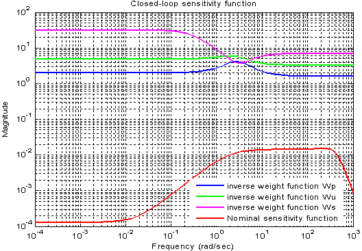
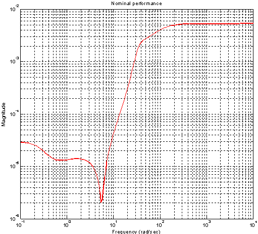
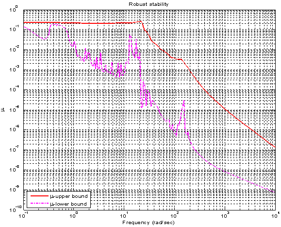
 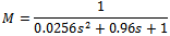 Synthesize the controller K∞ to make transfer function from disturbance to error minimum. For all MIMO systems for γ < 4 it can be shown theoretically that controller K∞ does not change shapes of singular values[19]. The robust stability is achieved without significant degradation in original characteristics. If γ > 4 then readjust the weight matrix. The controller is synthesized and stability margin (emax) calculated is 0.40851. The gamma value obtained is 2.44792 which satisfies stability margin. Figure 14 shows the frequency response of initial plant and shaped plant.The sensitivity function of the closed loop system is shown in Figure 15. It can be see that requirement of disturbance attenuation is satisfied[18]. The nominal performance is analyzed and it is 0.0053998 as shown in Figure 16. The frequency response of structured singular values for case of robust stability is shown in Figure 17. The maximum value of μ obtained is 0.25883 which means that stability of closed loop system is preserved under all perturbations that satisfy
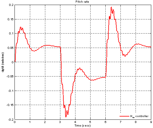
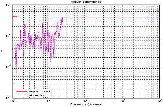
  [12]. The frequency response of μ for the case of robust performance analysis is given in Figure 18. The peak value of μ is 0.41893 which shows that robust performance is achieved and in higher frequency range it maintains constant value.Figure 19 shows the transient response of the closed loop system with designed 2 DOF H-∞ loop shaping controller for step signal with magnitude
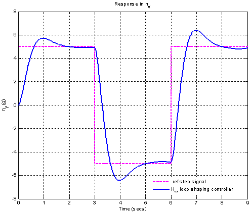
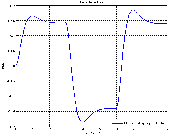
  which corresponds to change in normal acceleration. The overshoot is found to be 14.72%and corresponding settling time is 2.23 sec. The fins deflection obtained is 0.1617 rad. ( 9.27°) as shown in Figure 20. The pitch rate variation obtained is 0.1 (rad/sec) as shown in Figure 21.
 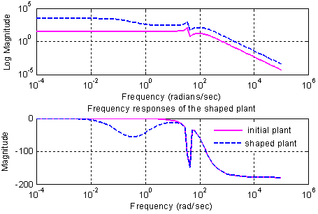 | Figure 14. Frequency response of initial plant and shaped plant for H-∞ loop shaping controller |
 | Figure 15. Closed loop sensitivity function for H-∞ loop shaping controller |
 | Figure 16. Nominal performance for H-∞ loop shaping controller |
 | Figure 17. μ- Robust stability for H-∞ controller loop shaping controller |
 | Figure 18. Robust performance for H-∞ loop shaping controller |
 | Figure 19. Acceleration response for H-∞ loop shaping controller |
 | Figure 20. Fins deflection response for H-∞ loop shaping controller |
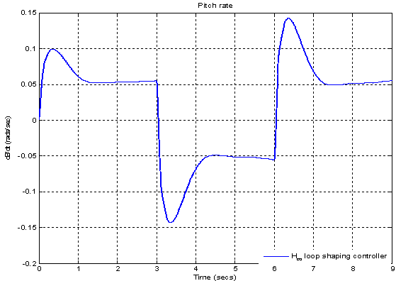 | Figure 21. Pitch rate response for H-∞ loop shaping controller |
4.3. Comparison and Limitations of Two Approaches
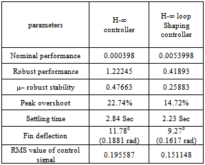
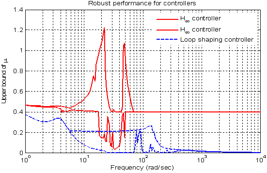
The comparison of closed loop system with H-∞ and H-∞ loop shaping controllers begins with robust stability and performance analysis. To achieve robust stability it isnecessary that the μ values are less than 1 over the frequency range. In Figure 22 we compare the structured singular values, for the robust stability analysis, of the closed-loop systems with both controllers. It shows that H-∞ loop shaping controller achieving better result.Table 2. Comparison of 2 controllers parameters
 |
| |
|
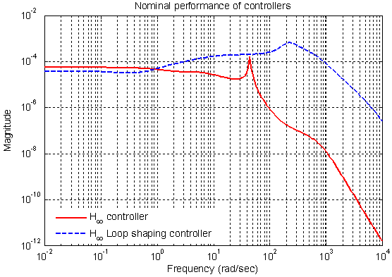
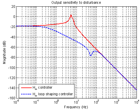
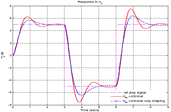
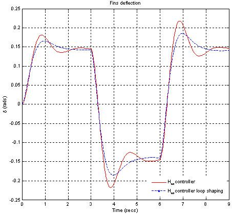
The comparison of nominal performance of twocontrollers is shown in Figure 23. In case of H-∞ loop shaping controller performance is slightly more than H-∞ controller. The slightly larger magnitude over the low frequencies leads to an expectation of steady state errors. The robust performance is also computed as shown in Figure 24. It shows that H-∞ loop shaping controller achieves better performance than H-∞ controller in low frequency range. The output sensitivity to disturbance is less in H-∞ loop shaping approach as shown in Figure 25. Further we can reduce output sensitivity to disturbance by using high gain values in pre filter design. Transient response of controller is shown in Figure 26. The peak overshoot is reduced in H-∞ loop shaping approach also response is less oscillatory but settling time is not reduced to large extent. As shown in Figure 27 fins deflection is reduced it shows longitudinal stability is improved in H-∞ loop shaping approach. Reduction in pitch rate is also achieved by H- ∞ loop shaping controller as shown in Figure 28. The RMS value of control signal related to fuel consumption. As value decreases proportionally fuel consumption reduced. RMS value is less in H-∞ loop shaping approach so using H-∞ loop shaping controller fuel consumption reduced. Table 2 shows comparison of performance parameters of two controllers.Figure (22) to (28) shows comparison of parameters of 2 controllers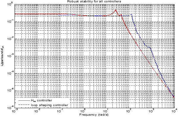 | Figure 22. μ- Robust stability for both H-∞ and H-∞ loop shaping controller |
 | Figure 23. Nominal performance of H-∞ and H-∞ loop shaping controller |
 | Figure 24. Robust performance for H-∞ and H-∞ loop shaping controller |
 | Figure 25. Output sensitivity for H-∞ and H-∞ loop shaping controller |
 | Figure 26. Response for acceleration for H-∞ and H-∞ loop shaping controller |
 | Figure 27. Response for fins deflection for H-∞ and H-∞ loop shaping controller |
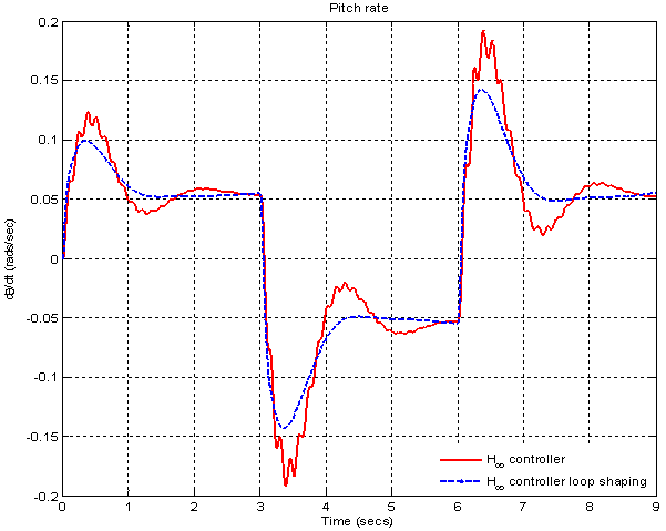 | Figure 28. Pitch rate for both H-∞ and H-∞ loop shaping controller |
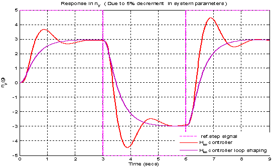 | Figure 29. Acceleration response due to 5% decrement parameters |
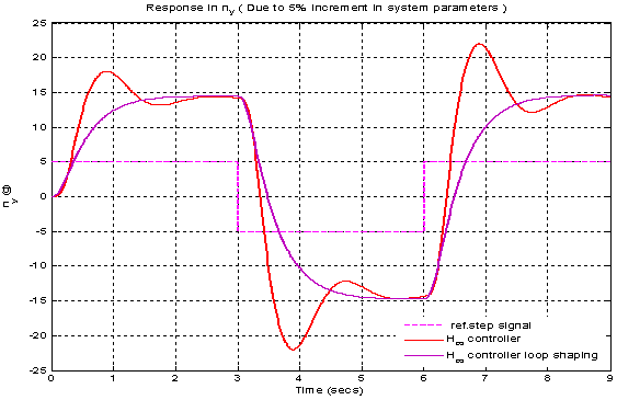 | Figure 30. Acceleration response due to 5% increment parameters |
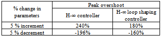
In above discussion controllers are designed andcompared their performance results. Every controller has its specific operating range and depends upon system parametervariation. In above system 5 % change in system parameters ,the controller fails. Table 3 shows peak over shoot. The responses are shown in Figure 28 and 29.Table 3. Effect on change in peak overshoot
 |
| |
|
From above table it shows peak overshoot exceeds it maximum limit. So for our controller we can vary system parameters up to 1% obtaining desired value in range .
5. Conclusions
A rocket model is developed in which pitch rate control is analyzed and simulated. The pitch rate control problem is related to the longitudinal stability of the rocket. According to result obtained from simulation it can be seen thatlongitudinal stability is improved using 2 DOF loop shaping controller.Due to presence of uncertain parameters the derivation of the uncertainty model required and heavy computations are demanded. That is the main reason why it is necessary to investigate the parameter importance with respect to the robustness performance and an objective is to reduce their number to an acceptable value. However, in the evaluation of the design, it is better to take into account all the possible uncertainties to ensure a satisfactory design in a present case. Here 15% uncertainties in parameters are taken.The performance of closed loop system using H-∞ loop controller is evaluated .The model facilitates γ iteration method for solving Ricatti equation for H-∞ controller design The performance of the closed loop system using H-∞ loop shaping controller is further evaluated. The application of a 2 DOF H- ∞ loop shaping controller in pitch rate auto pilot design shows that it is better in robustness and reduces control efforts without the degrading performance. Actuator efforts are critical consideration in the rocket auto pilot design since they invoke how quickly actuator command limiting is invoked. The pitch rate reduced and reduction in fins deflection shows that actuator efforts are reduced.
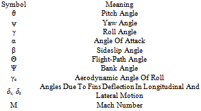
Nomenclature
References
| [1] | Zames G.(1981) “Feedback and optimal sensitivity model reference transformation, multiplicative semi norms and approximate references.” IEEE Transaction On Automatic Control AC-23 (1981), 301-302 |
| [2] | Doyle J., Glover K, Khargoeker P., and Fracis B (1989) “State space solution to standard H2 and H∞ control problem ” IEEE Transaction On Automatic Control 34 (1989), 831-847 |
| [3] | Glover k, Limebeer D, Doyle j, Kasenally E.M, and Sofonov M, (1991) “A characterization of all solutions to four block distance problem” SIAM Journal of control and optimization , 29 (1991) 283-324 |
| [4] | Reichert R T (1989) “Application of H∞ control to missile autopilot design” In Proceedings Of AIAA Guidance , Navigation And Control Conference , 1989 1065-1072 |
| [5] | McFarlane, D.C., and K. Glover, "A Loop Shaping Design Procedure using Synthesis," IEEE Transactions on Automatic Control, vol. 37, no. 6, pp. 759– 769, June 1992. |
| [6] | George m. Siouris “Modern missile guidance and control” springer – verlag .2004 (e-book) |
| [7] | Brodsky, S.A.; Aro, H.O (2011) “Application of robust control for attitude stabilization of supersonic winged rocket” IEEE Transaction On Control System, 978 – 1 – 4244 – 9616 - 7/11,2011 |
| [8] | J.Blaklock “ Automatic control of Aircraft & missiles ”. John wiley & sons. 2004 |
| [9] | Jack E. Nelsen “Missile Aerodynamics” Mc Graw Hill Publications 1960 |
| [10] | D.W.Gu , P. Peter “Robust control engineering design with MATLAB” .springer – verlag, 2005 1st Edition |
| [11] | S.Skogested, I.Postlethwaite “Multivariable feedback control system ” wiley & sons .2001 |
| [12] | M Green “Linear robust control” chapter 6: Full information about H-∞ synthesis. Dover publication .1998 |
| [13] | Mark .R. Tucker.and Daniel Walker.” H-∞ mixed sensitivity “, Robust flight control- Design challenge, leacture notes in control and information science, Springer- Verlag 2000 |
| [14] | Yang S M and Huang H “ Application of H-∞ control to missile auto pilot design” IEEE transaction on Control system 0018-9251/03 |
| [15] | R. Sobhani “ Nonlinear Digital Robust controller for UAV”, IEEE Aerospace conference 1-4144-0525-4/2007 |
| [16] | Sun Jie, Yang Jun “ Robust flight control law development for Tiltrotor conversion” IEEE 2009 International conference on intelligent human machine system and cybernetics 978/0-7695-3753-8/09 |
| [17] | Mingyun L V, Yanpenh Hu” Attitude control of unmanned helicopter using H-∞ loop shaping method” IEEE Transaction on Mechatronics sciences 978 – 1 – 61284 – 722 - 1/11 ,2011 |
| [18] | J.Gadewadikar, F.L.Lewis, Kamesh Subbarao and Ben M. Chen. “Structured H∞ Command and Control-Loop Design for Unmanned UAV”. Journal Of Guidance, Control, And Dynamics. Vol. 31. No. 4, July-August 2009. |
| [19] | J. Gadewadikar, F. L. Lewis, Kamesh Subbarao and Ben M.Chen.Attitude “Control System Design for Unmanned Aerial Vehicles using H-∞ and Loop-shaping Methods.” 2007 IEEE International Conference on Control and Automation. Guangzhou, CHINA May 30 to June 1,2007. |
| [20] | K Glover and R Hyde “H-∞ Loop shaping design for Flight”, Chapter 29 Robust flight control- Design challenge, lecture notes in control and information science, Springer- Verlag 2000 |
| [21] | T Chelaru, C Barbu “ mathematical model and technical solution for multistage sounding rocket” IEEE proceedings on international conference on applied mathematics and simulation, modeling 2009,978-960-474-147-2/0.9 |
 Abstract
 Reference
 Full-Text PDF
 Full-text HTML