1. Introduction

In the early 1980s, the US Air Force initiated a study called the DMICS with the objective of developingmethodologies for the design of IFPC laws for an advanced tactical aircraft[1]. Two very different approaches to IFPC designwere developed as a result of this study. These methods are a centralized approach, which consists of designing a "global" integrated compensator considering the fully integratedsystem as one high-order system[2], and a decentralizedhierarchical approach, which consists of partitioning the integrated system into loosely coupled subsystems and then designing separate controllers for the sub-systems such that some high-level performance criterion is met[3].

Owing to bilateral effects between the aircraft engine and body, separate optimization of propulsion and body might cause suboptimal system performance. Therefore, IFPCparameters should be tuned and optimized simultaneously. One of the complexities of IFPC design is simultaneouscontrollers gain tuning. The traditional approaches for the tuning of the control parameters, such as manual tuning approaches, are based on trial and error and may not result in an optimized engine and body performance. Consequently, the tuning process for the controller parameters is viewed as an optimization problem. Due to the nonlinearity and theswitching nature of the industrial GTE control strategy[4], as well as to complexity of gain tuning for the flight controller,gradient - based optimization methods have weak performance for gain tuning. As a result, this problem requiresanon-gradient optimization technique. In this study, the PSO is investigated for simultaneous tuning of the IFPC parameters in order to achieve an improved performance for the engine and body. In addition, the effect of neighbor acceleration on PSO results is studied.

PSO is presented by James Kennedy and R. C. Eberhart in 1995. This algorithm is based on the simulation of social behavior of birds flocking, fish schooling and herds of animals to adjust to their environment, find rich sources of food, and keep away from predatory of other animals by using an “information sharing” and “social cognitiveintelligence”[5, 6]. This algorithm generates a set of solutions in a multidimensional space randomly, which represent the initial swarm. This initial swarm contains particles that move in the space and search for the best global position. Iterations will be continued until the best global position is reached. After presentation of PSO by Eberhart, further researches areintroduced which modify the method and for faster convergence using adaptive PSO algorithm and neighbor acceleration effect[6-13]. In the aerospace field, the PSO method is used for parameterization of airfoils shape and its application in aerodynamic optimization[14]. Also, Praveen andDuvigneau applied the PSO to aerodynamic shape design. They illustrated that the use of mixed evaluations by metamodels / CFD can significantly reduce the computational cost of PSO while yielding optimal designs as good as those obtained with the costly evaluation tool[15]. Moreover, Bessette and Spencer successfully employed the PSO for space trajectoryoptimization[16, 17]. In 2012, Montazeri et.al used the PSO method for a jet engine Min-Max fuel controller design in order to reduce the fuel consumption and response time of a turbojet engine[18].

This paper applies the PSO in the IFPC gain tuning problem for the first time. For this purpose, an integrated flight and propulsion model is firstly developed in order to simulate the bilateral effects between the engine and body. The model consists of a 6 D.O.F nonlinear flight simulation which is derived from the equations of motion andaerodynamic equations, and a turbojet engine Wiener model which is confirmed by experimental data. The structure of the GTE fuel controller is then described based on an industrial fuel control strategy. A conventional glide slope control as well as a velocity control is also designed for the flight control system. Subsequently, the simultaneous tuning of the IFPC parameters is formulated as an optimization problem based on the PSO approach. For this optimization problem, the objective function is defined to minimize the PLA tracking error and oscillation of the operational parameters for the engine as well as the glide slope tracking and smooth variation of velocity for the body. Moreover, the effect of neighbor acceleration on PSO results is studied. Finally, the results of the PSO with and without neighbor acceleration factor are compared with the DP and the GA results to investigate the effectiveness of the proposed technique for IFPC gain tuning problem.

2. Integrated Flight and Propulsion Simulation

In order to perform the optimization of the aircraft GTE and body controllers in a practical manner, it is necessary to simulate these two systems simultaneously. This is because of the bilateral effects between the engine and the body in various flight conditions. In other words, separateoptimization of the aircraft engine or flight controllers may not satisfy the safe operation of the aircraft in various operatingconditions. To achieve this purpose, a combined dynamicsimulation consisting of both engine and flight is needed. In this section, simultaneous modeling of the engine and flight simulator is developed to evaluate the performance of the controllers.

2.1. GTE Modeling

The turbojet is the simplest form of gas turbine in that the hot gases generated in the combustion process escape through an exhaust nozzle to produce thrust. The main components of a basic GTE are shown in Figure1[19].

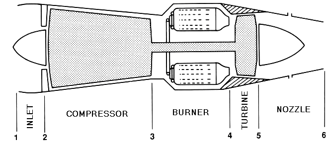Figure 1. Schematic of a basic GTE

Modeling of a GTE in order to design a controller usually carried out with transfer function or simplifiedthermodynamic models. Also block-structure model is used extensively for this purpose. Block-structured systems are systems that can be represented by interconnections of linear dynamic models and static nonlinear systems. The Hammerstein model shown in Figure2 (a) consists of the cascadeconnection of a static nonlinearity followed by a linear time-invariant system. Hammerstein models are usually used toapproximate systems, where the nonlinearity is caused only by the variation of dc gain with input amplitude. These models have constant dynamic behavior regardless of the input amplitude. It thus seems that Hammerstein models are not appropriate for nonlinear gas turbine modeling since the dynamics of the engine changes with the input amplitude. The Wiener model shown in Figure2 (b) consists of a linear dynamic element in series with a static nonlinear part. Unlike Hammerstein models, the nonlinearity in Wiener models is caused by the variation of the system static and dynamic characteristics with input amplitude. Wiener models thus seem to beappropriate candidates for nonlinear gas turbine modeling[20].

Figure 2. Nonlinear model structures: (a) Hammerstein (b) Wiener

In this paper, a Wiener model is developed for fuel controller design. This model consists of a first order transfer function as a linear time invariant part and look-up-tables as nonlinear static part. The linear time invariant part simulates the engine lag, whereas the static nonlinear part gives details about the relationship between the fuel flow and the engine parameters such as rotor speed, compressor pressure ratio, exhaust gas temperature and thrust. All of the engine model parameters are taken from the data obtained by experimental tests performed on the engine. More details about the engine modeling can be found in[21-23].

Figure3 compares the simulation results with the experimental data. The good agreement between the results support the simulation model used in this study.

Figure 3. Comparison between GTE simulation and experimental results

2.2. Flight Simulation

The flight mathematical model used in this study is a nonlinear representation of an aircraft with rigid body. The rigid body motion is modeled using six nonlinear force and moment equations and six kinematics equations. So the aircraft dynamics are modeled as a set of 12 first-order coupled nonlinear differential equations:

(1)

The state vector is defined the same as the output vector and can be represented as:

(2)

where:

u, v, w: air speed in body axes,

p, q, r: body roll, pitch and yaw rates,

: Euler orientation angles,

x, y, z: Position of the body center of mass,

And the control vector is defined as:

(3)

where:

The equations of motion are developed based on the assumption of the flat earth and constant mass properties. Also, aerodynamic forces and moments are obtained using stability and control derivatives based on an extensive theoretical works given in the format of a numerical look-up table.

In this research, the aircraft maneuver is in the vertical plane. So, the aircraft is maintained at a constant glide angle just by trimming the elevator deflection () provided by the flight path controller. Moreover, the aircraft forward speed (u) is controlled by the engine thrust (f) and the elevator deflection ().

2.3. Integration between Flight Simulation and GTE Model

The methodology used in this study for integration of flight simulation and engine model is to simulate the engine and airframe dynamics in a modular fashion to test both engine and body controllers for various altitudes, Machnumbers and pilot commands. The schematic of the integrated engine and airframe simulation is shown in Figure4.

3. Controller Design

In this section, the engine fuel controller as well as the body glide slope and velocity controllers are described based on the engine control modes and flight simulation control requirements. The structure of the controller is shown in Figure 5.

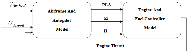Figure 4. schematic of engine model integrated with airframe model

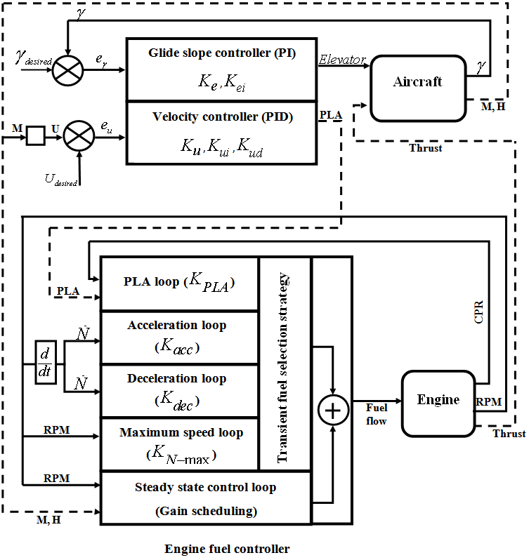Figure 5. Engine and aircraft controllers’ structure

3.1. GTE Controller Design

The control of a gas turbine engine can be summarized by three different control modes including a steady state control mode to satisfy the pilot command at steady-state condition, a transient control mode to regulate the time response of the engine, and a physical limitation control mode to fulfill the overspeed, over temperature and aerodynamic limitations.

In this paper, the fuel control system is designed based on an industrial strategy which divides the fuel flow into two parts including a steady state fuel flow and a transient fuel flow[4, 24]. The engine steady state fuel flow is defined for every equilibrium point. The steady-state controller isresponsible to meet the first requirement of the GTE control system i.e. the steady state control mode. In this study, this part of the fuel flow is calculated by a scheduling controller as a function of the engine rotor speed as shown in Figure5.

In addition to the steady-state control mode, a transient fuel flow is considered for the control of the engine transient performance as well as the engine limitations. Transient fuel flow is the variation of the fuel flow with respect to its steady-state value. In this study, the engine transient fuel flow is calculated using a min-max strategy where four proportional control loops are defined for calculation of the transient fuel flow including PLA loop, Deceleration loop, Acceleration loop and Maximum rotor speed loop as shown in Figure5. The proportional gains of these control loops named respectively.

3.2. Airspeed and Flight Path Control

Airspeed is a critical variable in the flight dynamics of an aircraft. The airspeed affects all of the aerodynamic forces and moments through the dynamic pressure. The airspeed controller uses a pitot tube to measure airspeed (u) and a PID controller to shape the control command which is sent to the throttle servo to adjust the propulsion power as follows:

(4)

Where and K_u, K_ui and K_ud are the PID controller gains for the airspeed control system that must be tuned.

In addition the glide path, controller uses the pitch angle (θ) from the gyro and a PI controller to form the control command which is sent to the elevator servo. The glide path controller has the same structure as the altitude hold controller except that the reference input is the glide path angle. So the Proportional-Integral controller of glide angle takes the following form

(3)

Where and K_e and K_ei are the PI controller gains for the glide angle control system that must be tuned.

Both throttle and elevator affect the speed but the short and long-term effects of each of these controls are quite different. The throttle essentially affects the speed only in the short term but the elevator changes the steady-state speed. The schematic of the aircraft controllers is shown in Figure5.

As it is observed in Figure5, there are 9 gains that must be tuned simultaneously for the engine and body control system.

3.3. Initial Gain Values

In order to select the initial gain values for the 9 previously mentioned control loops, a manual tuning process is carried out as follows:

For GTE controller:

− The engine PLA loop gain () is firstly initialized to achieve a preliminary response time. In order to improve the engine response time, is then increased until the process begins to oscillate. Then, in order to protect the engine against surge, the is changed until the maximum rotor speed derivative () is limited to an allowable value. After that, the is changed until the minimum rotor speed derivative () is limited to an allowable value. Consequently, the engine is protected against flameout. Finally, in order to keep the engine integrity, is increased until the overspeed in every condition are vanished without overshoot.

For body controllers:

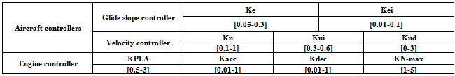
− The value of is increased to achieve an acceptable glide slope tracking. Next, the value is increased to eliminate the steady state error of glide slope tracking. Subsequently, the values of are changed in the same ways until a reasonable velocity tracking is reached for the aircraft.

The initial values obtained by the above process for a case study in Seal Level Standard (SLS) condition is shown in Table.1.

As mentioned earlier, the manual gain tuning process based on a trial and error manner may not result in an optimal controller for the aircraft and engine. Therefore, in order to achieve an improved performance for the engine and body simultaneously, the PSO method is proposed for IFPC gain tuning problem in this paper.

But, taking the iterative nature of PSO method into account, and since the IFPC controllers gain tuning problem is a 9-dimensional optimization problem, the design variable ranges play in important role in computational effort of the optimization algorithm. Therefore, these ranges are restricted by a manual sensitivity analysis. Table (2) shows the lower and upper bound for the design variables.

Table 1. Initial controller loop gains

Table 2. Solution space of IFPC gain tuning problem

4. Problem Formulation

In this section, application of PSO for optimization of the previously described controllers is explained. For this purpose, an overview of the method is firstly presented. The controller gain tuning procedure is then formulated as an optimization problem. Finally the PSO method is applied and the results are analyzed in the next section. The effect of neighbor acceleration factor on PSO results is also investigated in this paper.

4.1. Particle Swarm Optimization (PSO)

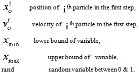
Particle swarm optimization is a method for performing numerical optimization without explicit knowledge of the gradient of the problem to be optimized. PSO is attributed to Kennedy, Eberhart and Shi[9] who are the founders of the field. Originally intended for simulating social behavior, the algorithm has been simplified after the particles have been observed to be performing optimization. The book byKennedy and Eberhart describes many philosophical aspects of PSO and swarm intelligence[5].

PSO shares many similarities with evolutionarycomputation techniques such as GA. The system is initialized with a population of random solutions and searches for optima by updating generations. However, unlike GA, PSO has no evolution operators such as crossover and mutation. In PSO, the potential solutions, called particles, fly through the problem space by following the current optimum particles. More details can be found in[6, 25, 26].

One of the main advantages of PSO is that the PSO has few parameters to adjust and therefore is easy to implement. PSO has been successfully applied in many areas including function optimization, artificial neural network training,fuzzy system control, and other areas where GA can be applied. This study suggests the PSO for IFPC optimization for the first time.

In this method, each particle refers to a point in a multi dimensional space whose dimension is related to the number of design parameters. The positions of points are changed in moves (iterations) with velocities which are calculated in each step. In the first step, positionand velocity for each point are generated randomly by upper and lower bounds of variable using the following equations:

(6)

(7)

Where

As mentioned earlier, the first population is distributed uniformly in the design space by this process. In the second step, PSO calculates new velocities to move the particles from positions at time k to new positions at time k+1. For calculation of new velocities, three terms are needed:

• Inertia term: each particle wants to continue its motion in its own current direction. This term is modeled bymultiplying the particle’s current velocity vector by a number called inertia factor.

• Cognitive term: taking the self confidence characteristic into account, each particle has a velocity in the direction of its own best position over all the previous and current steps, . This term is modeled by multiplying the difference between the particle’s current position and the best position over all previous iterations by a number called selfconfidence factor.

• Social term: each particle also gets effect from other particles. One particle may be affected by the best position of particles in the current swarm, , or by the best position of particles in its own vicinity, . In the first case the algorithm is termed gBest PSO (global best) and in the second case it is termed LBest PSO (local best). The social confidence factor is used to model this term.

PSO employs these three terms in addition to their corresponding coefficients to calculate new velocities for the next iteration using a random distribution function. The coefficients inertia factor, self confidence factor and social confidence factor show the effect of the current motion, particle own memory and swarm influence on the velocity vector of each particle, respectively.

The pseudo code of the procedure is as follows[11, 27]

For each particle

Initialize particle

End

Do

For each particle

Calculate objective value

If the objective value is better than the best objective value (pBest) in history

set current value as the new pBest

End Choose the particle with the best objective value of all and/or some of particles as the gBest and/or lBbest

For each particle

Calculate particle velocity

Update particle position

End

Based on the above explanation, the velocity update formula takes the form (8) for gBest PSO and form (9) for LBest PSO:

(8)

(9)

where:

Inertia factor,

Velocity of particle in the current motion,

Self confidence factor,

Social confidence factor (gBest),

Social confidence factor (LBest),

Position of particle in current motion,

Best position of particlein current and all previous iterations,

Position of the particle with best global objective at current iteration k,

Best local neighbor position in the current iteration.

In this paper, the PSO approaches, take the effects of both gBest and Lbest in the velocity equation. In this case, the approach is referred to as neighbor acceleration effect. This modification is implemented in order to improve the speed of convergence[20]. Consequently, the velocity update formula with neighbor acceleration effect takes the following form:

(10)

Using the updated velocities vectors calculated by equation (4) and (5), the position of each particle is changed through the following equation:

(11)

where is the Position of particle at step (k+1).

This algorithm is repeated until a stopping criterion is reached. This criterion may be an iteration number or a specified tolerance on the minimum improvement of the best global value.

A schematic view of the position update of a particle in gbest PSO and PSO with the neighbor acceleration effect is shown in Figure6. Moreover, in order to take both Lbest and gbest effect into account, a star social structure is defined for the swarm in this paper. Since all particles are connected using this topology, each particle can be affected easily by all the particles or by its own neighbor. In this paper,neighborhood is defined based on particles indices. In other words, neighbors of particle i_th, are particles (i+1)_th and particle (i-1)_th . Another definition for neighborhood is presented by Suganthan, based on Euclidean distance[28].

4.2. Objective Function

As mentioned earlier, the jet engine fuel controller, the aircraft glide slope and velocity controllers are designed to satisfy GTE control modes including steady state, transient and physical limitation control modes as well as aircraft control requirements. In other words, the objective of the engine controller is to drive the GTE to the pilot desired set-point with good tracking with respect to flight path and speed requirements. Also, the objective of the body controller is to track the desired glide slope based on the specified aircraft maneuver as well as smooth and reasonable variation of the speed with respect to safe operation of the engine. In both engine and body, the oscillation of parameters should be avoided. In addition, the engine must be protected from the physical limitations such as over speed, flame out, lean and rich blowout and surge in compressor. These terms are defined as penalty functions for the objective. Therefore, the objective function is formulated as follows:

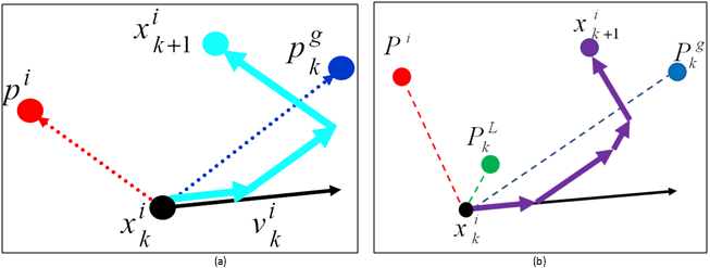Figure 6. PSO position updates (a): gbest PSO, (b): PSO with neighbor acceleration effect

(12)

where:

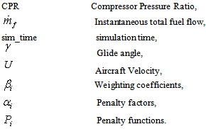In equation (12), the performance indices are normalized first and then weighted according to their importance by the coefficients of . In this paper all of these coefficients are assumed the same (0.25). The first and second terms in the equation (12) are related to the engine parameters. The first term guarantees the PLA tracking. It is worth mentioning that what the pilot usually wants to achieve while moving the thrust lever is to let the engine deliver a certain percentage of the thrust that is available at the current flight conditions[29]. Since thrust itself is not measurable in flight, the relative thrust command given by the PLA setting must be translated into a command change of a measured variable. The relative thrust corresponds very well to the CPR and this parameter can be used for thrust modulation in controller design. The second term in (12) is aimed at obtaining a smooth change in the fuel flow, which results in a smooth variation of the engine operating parameters.

The third and fourth terms in (12) are related to the aircraft glide slope tracking and the smooth variation of aircraft velocity respectively. The are termed to penalty factors tuned manually to achieve the reasonable results and are termed to physical limitation as mentioned earlier.

Moreover, the design optimization variables are the controllers loop gains including ,,, in engine controller, , in glide slope controller, , and in velocity controller as shown in Figure5. In other words, these 9 variables are going to be tuned using PSO in order to minimize the objective function of equation (12).

5. Optimization Results and Analysis

In this section, the result obtained from the gain tuning approach is studied in order to confirm the effectiveness of the PSO method for the optimization of IFPC performance. Subsequently, the effect of neighbor acceleration on the PSO results is analyzed and compared with the initial optimized controller. Moreover, the results obtained from theapplication of a GA method are compared with the PSO results. Finally, the engine and aircraft performance with the optimized controllers derived from PSO with and without the neighbor acceleration effect along with GA are investigated and compared in order to evaluate the effectiveness of the methods on the optimization of IFPC performance.

In this study, a computer simulation program is developed for a single spool turbojet engine integrated with a 6 D.O.F nonlinear flight simulation as a case study. Using each set of controller’s parameters, the time domain simulation is performed and the objective value is determined. The objective function is first evaluated by simulating the IFPC model considering a climb-cruise-landing maneuver as shown in Figure 7.

5.1. PSO Results

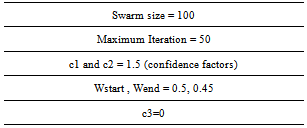
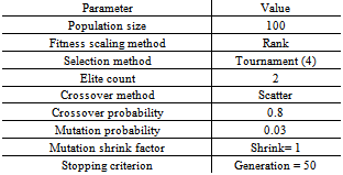
In order to achieve an improved performance, theoptimization process has been run in a trial and error manner with several PSO parameters to find the best set of parameters. The best results are achieved for the parameters presented in Table (3). It is worthwhile to mention that there are some heuristic methods in the literature to find the PSO parameters. A study about these methods as well as their theoretical limitations can be found in[30, 31]. As shown in Table (3), the inertia factor decreases each iteration in order to transform the exploration nature of the algorithm in the initial runs to exploitation nature in the final runs. The variation of this factor is linear as shown in Figure8. The confidence factors are set to 1.5 and the neighbor factor is set to 0 for gbest PSO. Moreover, the weight factors, are selected for the objective functions in equation (12). It means that the importance of the objectives is equal in the optimization process. Optimization is terminated in the prespecified number of generations.

Table 3. Parameters used in PSO

Figure 7. Simulated maneuver

Figure 8. The variation of the inertia factor

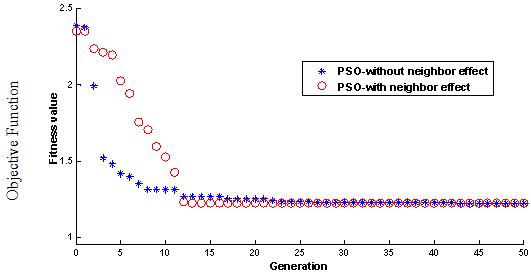Figure 9. The PSO optimization process history (average of 15 runs)

Figure 10. Objective function value for PSO (average of 15 runs)

In order to analyze the effect of the neighbor acceleration factor on the PSO results, the effect of the positions of the neighbor particles is also considered in this paper. For this purpose, the term with factor c3=1 is used in equation (10). Figure 9 shows the history of the objective function for both gbest PSO and PSO with neighbor effect. This Figure is derived from average of 15 runs of PSO with the Table (3) parameters. It is clear from Figure 9 that, when the effect of neighbor acceleration is considered on the velocity update, the PSO converges faster (12 generations with neighbor acceleration effect against 28 generations without it). The faster convergence for the PSO with neighbor effect is due to more information sharing among particles. In other words, the particles degree of freedom is increased using theneighbor acceleration factor. It should be mentioned that increasing or decreasing of c3 factor can increase or decrease the information sharing weight between the particles respectively. The value of c3=1 causes the best results for the in hand problem. More details can be found in[18].

Generally, the literature reports that the gbest PSOconverges faster than Lbest PSO because of better information sharing among the particles. The results of this paper show that the combined PSO (gbest PSO with neighbor effect) has better static convergence characteristics in comparison with gbest PSO for the problem at hand. Moreover, the neighbor effect gives a clustering character to the algorithm and prevents the solution from trapping in local optima.

Figure 10 shows the normalized objective function value respect to the value of initial controller (controller with the gains presented in Table (1)). This Figure shows that the PSO method improves the objective value and confirms the effectiveness of the approach. The values of the objective function obtained from PSO with and without neighbor effect are approximately the same (about 26% improvement in comparison with the initial controller).

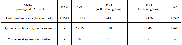
5.2. Comparison between PSO and GA

In this section, the PSO results are compared with the results obtained from the Genetic Algorithm (GA) in order to confirm the effectiveness of the proposed approach in optimization of IFPC gain tuning problem. The structure of simple GA used in this paper is composed by an iterative procedure through the five main steps: To start the algorithm, an initial population of individuals (chromosomes) is defined. A fitness value is then associated with each individual, expressing the performance of the related solution with respect to a fixed objective function (defined in equation (12)) to be minimized. Reproduction is then carried on as a process of generating a new population from the current population. The next step is selection, a mechanism for selecting the individuals with high fitness over low fitted ones to produce the new individuals for the next population. The variant used here is the roulette wheel method in which the probability to choose a certain individual is proportional to its fitness. Subsequently, crossover and mutation are applied to the population as GA operators. Crossover is the method of merging the genetic information of two individuals (parents) to produce the new individuals (children). The scattered crossover method is used in this study. Mutation is a probabilistic random deformation of the genetic information for an individual. This process can be handled by altering each gene randomly with a small probability. The positive effect of mutation is the preservation of genetic diversity and that the local maxima can be avoided. Following the evaluation of the fitness of all chromosomes in thepopulation, the genetic operators are applied to produce a new population. After repetitions of the above operations, the new set of strings is obtained. This ends an iteration of the GA. This process is iterated and new populations are produced until a termination criterion is fulfilled. The GA was also run several times with various parameters for achieving the best results. Since the GA has more parameters than PSO, setting the best parameters for GA runs is more complicated than for PSO. Table (4) shows the best parameters of GA for the IFPC controllers gain tuning problem. In addition, the population size, initial population and stopping criterion are set to the same values in PSO and GA in order to compare the two approaches more precisely. More details about the application of GA in aero-engine problem can be found in[32].

Table 4. Parameters used in GA

• Static convergence comparison

In order to investigate the ability of the proposed approach to find the global optimal solution, the dynamic programming (DP) method is also applied to the problem. The DP method works based on the principle of optimality. It should be mentioned that DP cannot give the controller parameters and only calculates the optimal control signal for the defined input PLA by breaking it down into simpler sub-problems in a recursive manner. The DP algorithm used in this paper is generated based on the theory presented by Dasgupta et al[33]. Table (5) compares the best objective value obtained from PSO and GA with DP. This table also shows the average of 15 runs. As it can be seen in this table, the objective value of the PSO is reasonably close to the objective value obtained from the global solution of DP. These results confirm that PSO provides almost the global optimal value for this problem. It seems that the GA method requires a parameters tuning process to achieve fitter results. Table (5) also compares the generation in which theoptimization algorithms find the final solution. As shown in this table, the PSO method converges faster than GA for the IFPC gain tuning problem. It confirms the effectiveness of the proposed approach for IFPC controller design. However, it is worth mentioning that regarding the time consumption of all applied methods, the methodology used in this paper cannot implemented in a real-time application.

Table 5. comparison between PSO and GA results (average of 15 runs)

Figure 11. Standard deviation of population for PSO and GA

● Comparison of computational effort

As shown in table (5), the PSO run time is less than GA because of fewer fitness evaluations in PSO. Taking the reduced number of parameters and the faster convergence of PSO into account, this table clearly demonstrates thesimplicity of the PSO algorithm that resulted into huge saving in the computational efforts, in comparison with othercomparatively old and well-established techniques for population based evolutionary computations like the GA. In addition, another advantage of PSO is that PSO has fewer parameters to adjust and therefore is easy to implement.

● Dynamic convergence comparison

In order to compare the dynamic convergence of the used optimization approaches, the standard deviation ofpopulation in each generation for the GA and PSO is plotted in Figure (11). These results are extracted from a typical run and it can be shown that this trend is similar for all runs. As shown in Figure11, the dynamic convergence of PSO is considerably better than GA because GA uses mutationoperator that increase the standard deviation.

The results presented in this section confirm theeffectiveness of PSO method in IFPC gain tuning as a real-world engineering optimization problem. The comparison between the PSO and GA results illustrates the relative merits of PSO from various points of view such as static and dynamic convergence and computational effort. Moreover, the PSO is easier to program in comparison with GA. In addition, taking the effect of both gbest and Lbest into account, leads to improving the PSO results considerably. Therefore, the PSO method is recommended for the IFPC simultaneous gain tuning problem. The effect of the optimization process on IFPC performance is presented in the next section.

5.3. Effect of Optimization on the IFPC Performance

The PSO changes the IFPC loop gains and simulates the engine and aircraft performance iteratively until the stopping criteria of the optimization problem are fulfilled. In order to verify and compare the effectiveness of the optimizedcontrollers, the performance of the PSO with and withoutneighbor acceleration effect is tested for the specified maneuver. These results are compared with the results obtained from simulation of the initial controller with the gains presented in Table (1). As mentioned earlier, a climb-cruise-landingmaneuver as shown in Figure7 is employed in this study.

Figure12 shows the variation of altitude during themaneuver. As shown in this Figure, the initial controller cannot satisfy the maneuver altitude tracking. Both of PSO methods give good results in aircraft altitude control.

Figure13 shows the variation of aircraft speed. As shown in this Figure, the steady-state error is eliminated by the PSO methods. However, the PSO results with neighbor effect are better than the PSO results without neighbor effect. The smooth variation of aircraft speed around the desiredmagnitude is also reached using the optimization method.

Figure 14 shows the glide angle tracking for the defined manuever using the initial and the optimized controllers. As shown in this Figure, the results obtained from PSO show fast and acceptable response to the glide slope change, whereas the initial glide slope controller has a little lag to follow the specified glide slope.

Figures 15 and 16 depict the engine performance. Figure 15 shows the PLA tracking of the GTE. This Figure shows that the results obtained from PSO outperform the initial controller.

Figure 16 shows the engine rotor speed in climb – cruise - landing maneuver. This Figure shows the ability of the optimization approach to achieve an efficient variation of RPM in this maneuver.

Figure 12. The variation of altitude through the maneuver

Figure 13. The variation of aircraft velocity through the maneuver

Figure 14. The glide angle tracking through the maneuver

Figure 15. The gas turbine engine PLA tracking through the maneuver

Figure 16. The gas turbine engine rotor speed variation through the maneuver

Figure 17. The 3-D maneuver

Figure 18. The glide angle and velocity tracking through the 3-D maneuver

Figure 19. The variation of gas turbine engine rotor speed and compressor pressure ratio through the 3-D maneuver

It can be observed from Figures.12-16 that both PSO without neighbor effect and PSO with neighbor effect outperform the initial controller. The response with PSO is much faster, with less overshoot and settling time compared to the initial controller. The responses of PSO with and without neighbor effect are almost similar, but the PSO with neighbor effect converges in fewer generations.

5.4. Reliability of Optimized Controllers

Finally, to confirm the reliability of PSO method in optimization of IFPC problem, the optimized controller is tested in a 3-dimensional challenging spiral maneuver as shown in Figure (17). This maneuver is carried on in 350 seconds. The optimized controller found by PSO with neighbor effect (in section 5.1) is used for this simulation.

Figure (18) shows the aircraft parameters through the maneuver. As shown in this Figure, the optimized controller performs very well in tracking the glide slope as well as the desired velocity. This Figure proves the reliability of the optimized glide slope and velocity controller of the aircraft.

Also, Figure (19) shows the engine parameters through the maneuver. This Figure also shows the smooth variation of the engine CPR and RPM, which confirms the optimized operation of aero-engine as well as protection of the engine against physical limitations.

Figures 18 and 19 confirm the reliability of PSO as a swarm intelligence optimization method in simultaneous gain tuning of integrated flight and propulsion control as a challenging real-word optimization problem. Finally, it should be mentioned that the tuned controller with frozen gains performs well up to 7000 meter as shown in Figure17. Future studies can focus on other altitudes and also on noise rejection and load disturbance attenuation.

6. Conclusions

In this paper, application of PSO techniques is presented for the simultaneous IFPC gain tuning. PSO is applied to optimize a long term objective function in order to achieve a simultaneous acceptable performance for both engine and aircraft. The results show that the PSO optimized controller outperforms the initial controller in all objective function terms. Moreover, comparison between PSO and GA results confirms the effectiveness of PSO as an appropriatecandidate to optimize the IFPC problem in comparison with other non-gradient based optimization methods like conventional GA. In addition, the influence of the neighbor acceleration effect on the PSO performance is investigated in this paper. The results show that the neighbor acceleration factor has a considerable effect on the convergence rate of the PSO process. For this purpose, a computer simulation isdeveloped for a single spool turbojet engine integrated with a 6 D.O.F nonlinear aircraft model to evaluate the objective function and to investigate the effectiveness of the approaches. For this optimization problem, the objective function isconsidered as a combination of the weighted PLA tracking and smooth response for the engine as well as glide slopetracking and velocity control for the aircraft. The results show that PSO can be used successfully for the optimization of the IFPC parameters. The PSO has the advantage of fewerparameters to adjust which makes it easy to implement. Finally, the reliability of the optimized controller is illustrated using a 3-D spiral maneuver. In other words, the results of this paper show the successful application of PSO in an important aerospace control problem.

Abbreviations

Particle swarm optimization (PSO)

Integrated flight and propulsion control (IFPC)

Gas turbine engine (GTE)

Pilot lever angle (PLA)

Design Methods for Integrated Control Systems (DMICS)

Dynamic programming (DP)

Genetic Algorithm (GA)

Proportional-Integral-Derivative (PID)

Degree of Freedom (D.O.F)

compressor pressure ratio (CPR)