1. Introduction

The turn of mechanical, aeronautical and civil design requires structures to become lighter, more flexible and stronger, so in recent years, the light plates have been widely used in various engineering applications, such as precision machinery, aircrafts, and vehicles[1]. These requirements cause the structure to be more easily influenced by unwanted disturbances, which may lead to vibration and some problems such as fatigue, instability, performance reduction, and may even cause damage to highly stressed structures. Therefore, it has attracted many researchers in fields of structural vibration analysis, damage detection, vibration and noise control[2-4].

From different kinds of control strategies consist of a purely passive control, a purely active control and a hybrid control[5],the use of active control techniques for the suppression of vibrations of very light structures is a very important target in many applications, where the additional masses of stiffeners or dampers should be avoided. Active techniques are also more suitable in cases where the disturbance to be cancelled or the properties of the controlled system vary with time[6].

In practice, any structure that deforms under some loading can be regarded as flexible structure and is a distributed parameter systems. This implies that vibration at one point is related to vibration at the rest of the points over the structure. Thus, it is desirable to use appropriate sensors and actuators. Piezoelectric sensors and actuators are extensively employed in many practical applications such as smart structures due to their lightness and their capability of coupling strain and electric fields. In order to control structural vibrations, piezoelectric sensors and actuators can be easily bonded on the vibrating structure[7].

In terms of the dynamic performance and active vibration control of plates, the high-efficient dynamic modelling and appropriate control law design are the two key points. So, in recent years researchers have used different kinds of modelling methods such as finite element methods[8, 9], finite difference methods[10, 11], modal analysis[12, 13], exact mathematical modelling[14, 15], experimental analysis [16, 17], and system identification[18, 19]. Also, various types of controller design methods such as velocity feedback control[20], high gain feedback regulator[21], linear quadratic regulator (LQR) approach[22], control[23], control[24], neural network control[25], fuzzy logic control[26], and intelligent algorithms[27] have been studied by former scientists. In additions, some others evaluate the performance of control algorithms in vibration suppression of flexible structure experimentally[28].

In this work, an accurate model of a homogeneous plate with special boundary conditions is derived by using of modal analysis. The derived formulation can calculate transfer function from actuators voltages to sensors voltages for all plate’s modes. The obtained model has infinite number of modes, so some first modes are considered as nominal system and remaining high frequency modes are left as a multiplicative unstructured modelling uncertainty. After modelling multiplicative uncertainty, the augmented uncertain plant is obtained an optimal robust controller is designed using µ-synthesis with DK-iteration. Then, a multi-objective robust controller is designed based on the augmented plant composed of the nominal model and its accompanied uncertainty. Finally, using an algorithm for µ-analysis, robust and nominal performances of designed controllers are achieved for perturbed plants and results were compared.

2. Dynamic Modelling of Structure

To design a controller that suppresses the structural vibration, one should implement an accurate model that shows the dynamic response of the flexible structure in different environmental conditions and disturbances. There are many methods, as mentioned before, to obtain dynamic model of structures. However, in homogeneous structures with special boundary conditions such as simply supported one we can use modal analysis to attain accurate models[26]. Using the modal analysis procedure, the plate transverse deflection at any point with respect to time position function can be modelled. This function can be expanded as an infinite series, as[29]

(1)

where, , is referred to as the modal displacement or generalized coordinate and is the plate displacement modal amplitude. The mode numbers in the directions of and are represented by and , i.e. for our case .

Because of wide applications of plates in aerospace and other applied area, here a smart plate is considered to modelling.

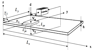Figure 1. A thin simply supported plate with actuator, sensor and control unit

Consider a thin plate with dimensions of as shown in Figure 1. Piezoelectric actuator and sensor layers of dimensions are bonded to the surface of the plate on both sides. The partial differential equation that governs the dynamics of the thin plate is[30]

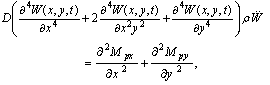(2)

where the term is the flexural rigidity of the plate, and and are defined as the moments generated by the piezoelectric actuating layer per unit length along and directions. For the plate, represents the mass per unit area, is the thickness, while and are the Young’s modulus and the Poisson’s ratio, respectively.

For a simply supported plate, the following boundary conditions hold:

(3)

The eigenfunction that satisfies these boundary conditions and the eigenvalue problem can be shown to be a double-sinusoidal function[30], as

(4)

while the natural frequencies of the thin plate with the above boundary conditions satisfy[30]

(5)

A common arrangement for the piezoelectric elements is the two-dimensional antisymmetric configuration [30]. This configuration assumes that the piezoelectric elements are larger in the and directions compared to the direction, i.e. . Since the piezoelectric layers are symmetrical when a voltage is applied across the electrodes of the actuating element, it induces equal surface strains to the plate in the x and y directions, i.e. .

From the modal analysis solution, the transfer function from the applied disturbance voltage to the plate deflection can be written as

(6)

where is the damping coefficient, which is normally determined experimentally, but generally is obtained by[31]

(7)

where and are two positive constant. is based on the properties of the plate and the piezoelectric actuating layer:

(8)

where is the strain constant and is the thickness of the piezoelectric layer. is a geometric constant which depends on the properties of the actuating layer and the plate[30]:

(9)

Here, and are the Young’s modulus and the Poisson’s ratio of the piezoelectric layer. Furthermore, the function term depends on the location of the actuator layer on the plate surface, such that[32]

(10)

Note that and are the coordinates of a corner of the actuating layer, as shown in figure 2, such that and .

The transfer function between the applied voltage and the shunting layer output voltage , can also be found as

(11)

where[32]

(12)

Using the same assumptions as the actuator layer, the sensor layer geometric constant can be determined as

(13)

where is the electromechanical coupling factor, is the stress voltage coefficient, and is the capacitance of the sensor piezoelectric layer.

3. Controller Design

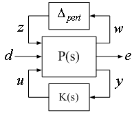
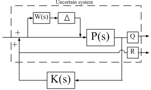
Suppose that control input and disturbance enter through the same channel. Therefore, the closed-loop system by considering multiplicative uncertainty will be as Figure 2.

Figure 2. Closed-loop system with multiplicative uncertainty

where P(s) is the nominal plant, K(s) is desired controller, ∆ is a stable transfer function, where and W(s) is the weighting function for multiplicative uncertainty, that is satisfies following equation:

(14)

where is the transfer function of the real system, by considering all or some of higher modes.

3.1. µ-Synthesis

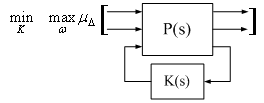
In order to apply the general structured singular value theory to control system design, the control problem should be recast into the linear fractional transformation (LFT) setting as in Figure 3.

Figure 3. LFT description of control problem

where is the open-loop interconnection and contains all of the known elements including the nominal plant model, performance and uncertainty weighting functions. The block is the uncertain element from the set , which parameterizes all of the assumed model uncertainty in the problem. is the controller. Three sets of inputs consist of perturbation , disturbances , and controls enter . And three sets of outputs consist of perturbation outputs , errors , and measurements are generated.

The set of systems to be controlled is described by the LFT as

(15)

The design objective is to find a stabilizing controller , such that for all such perturbations , the closed-loop system is stable and satisfies

(16)

But,

(17)

Therefore, the design objective is to find a nominally stabilizing controller , such that for all , , the closed-loop system is stable and satisfies

(18)

Given any , this performance objective can be checked utilizing a robust performance test on the linear fractional transformation. The robust performance test should be computed with respect to an augmented uncertainty structure. The structured singular value provides the correct test for robust performance. achieves robust performance if and only if

(19)

The goal of µ-synthesis is to minimize over all stabilizing controllers , the peak value of of the closed-loop transfer function . More formally,

(20)

This aim is shown in Figure 4.

Figure 4. µ-Synthesis concept

For tractability of the µ synthesis problem it is necessary to replace with the upper bound.

For a constant matrix M and an uncertainty structure , an upper bound for is an optimally scaled maximum singular value,

(21)

where is the set of matrices with the property that for every , . Using this upper bound, the optimization in equation is reformulated as

(22)

The D minimization is simply an approximation to . is chosen from the set of scalings, , independently at every . So,

(23)

, means a frequency-dependent function D that satisfies for each . The general expression is noted as , giving

(24)

Consider a single matrix , and a complex matrix M. Suppose that U is a complex matrix with the same structure as D, but satisfying . Each block of U is a unitary (orthogonal) matrix. Matrix multiplication by an orthogonal matrix does not affect the maximum singular value, hence

(25)

Therefore, replacing D by UD does not affect the upper bound. Using this freedom in the phase of each block of D, the frequency-dependent scaling matrix can be restricted to be a real-rational, stable, minimum-phase transfer function, , and not affect the value of the minimum. Hence the new optimization is

(26)

This optimization is currently solved by an iterative approach, referred to as D-K iteration. A block diagram depicting the optimization is shown in Figure 5.

To solve optimization problem, in the first stage consider holding fixed at a given, stable, minimum phase, real-rational . Then, solve the optimization

(27)

Define to be the system shown in Figure 6.

So, the optimization is equivalent to

(28)

Since is known at this step, this optimization is precisely an optimization control problem. The solution to the problem is well known and involves solving algebraic Riccati equations in terms of a state-space model for .

In the second stage with K held fixed, the optimization over D is carried out in a two-step procedure:

-Finding the optimal frequency-dependent scaling matrix D at a large, but finite set of frequencies (this is the upper bound calculation for µ).

-Fitting this optimal frequency-dependent scaling with a stable, minimum-phase, real-rational transfer function .

The two-step procedure is a viable and reliable approach. The primary reason for its success is the efficiency with which both of the individual steps are carried out.

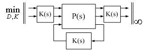Figure 5. Replacing µ with upper bound

Figure 6. Replacing rational D scaling

3.2. LMI-Based Design

For robust stability, we should have, where is transfer function from to when ∆ is removed. Therefore, the performance is appropriate for applying robustness in order to model uncertainty. However, to handle stochastic aspects such as measurement noise and random disturbance, the performance is functional. For appropriate disturbance rejection and control effort should be minimized, where Q and R are two weighting function that indicate relative importance of disturbance rejection and control effort. For minimizing performance index, we should minimize , where is a bounded norm exogenous disturbance. The transient response of a linear system is well known to be related to the locations of its closed-loop poles. So, closed-loop system poles should be located in a appropriate region of left half plane.

is equivalent to [24], so the above system can be shown as Figure 7.

Now assume that a state space representation of the open-loop system in Figure 7 (by ignoring K(s)) is

(29)

where and are control input and disturbance, respectively.

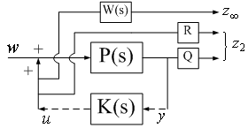Figure 7. Desired input and outputs of augmented plant

Our objective is to design a dynamic output-feedback controller with the state space realization

(30)

where is the state variable of the controller.

Therefore, the closed-loop corresponding system state-space equations containing performance and robustness channels will be as bellow

(31)

Our three design objectives can be expressed as follows:

Performance: the closed-loop RMS gain from to does not exceed if and only if there exists a symmetric matrix such that

(32)

This performance is used to minimize (closed-loop gain from disturbance to output channel)

Performance: the norm of the closed-loop transfer function from to does not exceed if and only if and there exist two symmetric matrices and such that

(33)

Pole placement: the closed-loop poles lie in the LMI region

(34)

With and if and only if there exists a symmetric matrix satisfying

(35)

For tractability in the LMI framework, we must seek a single Lyapunov matrix

(36)

That enforces all three sets of constraints. Factorizing as

(37)

And, introducing the change of controller variables[33]:

(38)

The inequality constraints on are readily turned into LMI constraints in the variables , , , , , and [34, 35]. This leads to the suboptimal LMI formulation of our multi-objective synthesis problem, which is defined as:

Minimize over variables , , , , , , and satisfying:

(39)

Given optimal solutions of this LMI problem, the closed-loop and performances are bounded by

(40)

4. Simulation, Results and Discussion

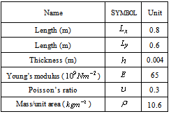
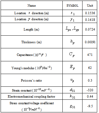
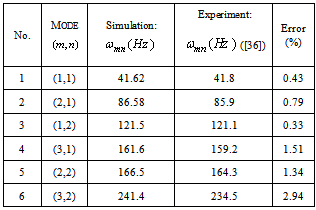
For designing a controller, a structure consists of aluminium plate simply supported at all edges with two identical piezoelectric patches are used as an actuator and a sensor, respectively. The patches are attached symmetrically to either side of the plate, thus collocating the actuator and sensor. The plate model is shown in Figure 1. A model of the structure is obtained via modal analysis technique. Dimensions and physical properties of the plate and the piezoelectric layers are summarized in Tables 1 and 2.

For verifying the obtained model, Table 3 shows the comparison of the six lowest resonant frequencies from the simulation and experiment results that is represented in[36] for two similar piezoelectric laminate plates. It is observed that the errors of the model in predicting the actual resonant frequencies vary around a few percent but the differences between the simulation and the experiment increase at higher-frequency modes. So, considering high frequencies as uncertainties eliminates this increasing error.

Table 1. Parameters of the simply supported plate

Table 2. Piezoelectric actuator and sensor parameters

Table 3. Six lowest natural frequencies of the plate

The frequency response of the plate deflection to the actuator voltage for the case (,) is shown in Figure 8.

First two shape numbers (,) of this plate are considered as nominal model and other eight numbers (,) remain as unstructured uncertainty. So, bode diagram of the nominal model will be as figure 9.

In addition, a weighting function for multiplicative unstructured uncertainty that satisfies is considered. Figure 10 shows the weighting function relation to real system.

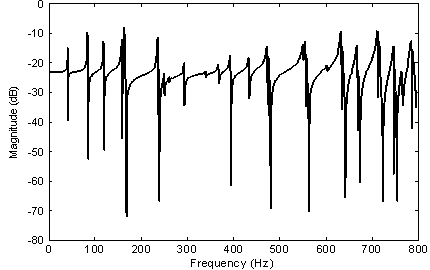Figure 8. Frequency response of modeled plate

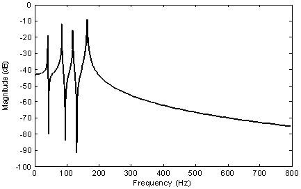Figure 9. Bode diagram of the nominal model

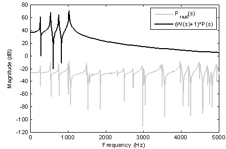Figure 10. The relation of weighting function to real system

4.1. µ-Synthesis

For designing a robust controller for mentioned smart structure using µ-Synthesis, uncertain system by multiplicative uncertainty is considered as figure 11. Two outputs consist of sensor voltage and actuator voltage by appropriate weights is considered.

Figure 11. Desired uncertain system used in µ-Synthesis

By considering and , using D-K iteration desired robust controller is obtained. This controller is of order 21. Comparison of frequency responses of closed-loop system and open-loop system is shown in Figure 12. This figure shows that the amplitude is reduced in the nominal model natural frequencies.

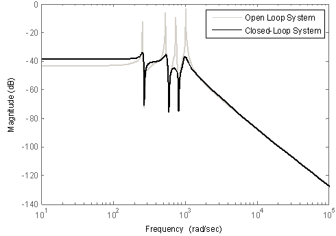Figure 12. Bode diagram of closed-loop system and open-loop system

Comparison of the impulse response of the closed-loop system with this controller and the impulse response of the open-loop system (Figure 13) shows the performance of the controller. This controller suppresses all vibration in less than 0.4 seconds.

Actuator voltage of this controller during the impulse response is plotted in Figure 14.

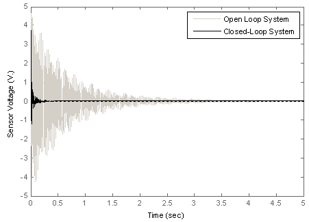Figure 13. Impulse response of the open-loop and closed-loop system

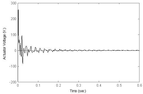Figure 14. Input control for impulse response of the closed-loop system

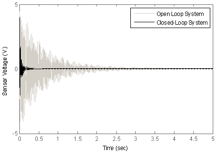
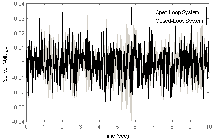Figure 15. Closed-loop system and open-loop system responses to a random disturbance

As one can see, the maximum amplitude of the actuator voltage is under 270 Volts.

Also, the open-loop and closed-loop responses to a random disturbance in duration of 10 seconds are compared in the Figure 15. Actuator voltage is shown in Figure 16, too.

The designed controller was mounted on the nominal plant. For investigation of the robust performance of the uncertain closed-loop system with the designed controller by structured singular value analysis Figure 17 is obtained. This plot shows upper/lower bounds of uncertain closed-loop structured singular values in frequency domain.

The performance margin is the reciprocal of the structured singular value and if the magnitude of the structured singular value were under unit, in all frequency range, the system has robust performance. Therefore, upper bounds from structured singular value become lower bounds on the performance margin and critical frequency associated with the upper bound of the structured singular value, here is. 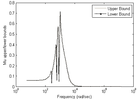In addition, the system can tolerate up to 140% of the modelled uncertainty without losing of desired performance. Note that robust performance guarantees robust stability of the uncertain system.

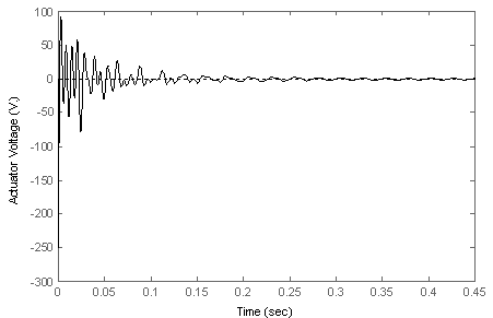
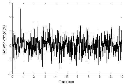Figure 16. Control input of closed-loop system in duration of a random disturbance

Figure 17. µ bounds of uncertain closed-loop system

4.2. LMI-Based Design

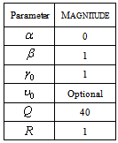
Now we can design desired controller by solving convex optimization problem that was formulated in (39). For obtaining an appropriate performance (robust stability) the magnitude of should be under unit, however it is not necessary to minimize it. But, for good performance we should minimize or norm from exogenous disturbance to performance index, and the relative magnitudes of Q and R determine the relative importance of disturbance rejection (vibration suppression) to control effort (actuator saturation). Then, the magnitude of the constants,, , , Q and R that imply to constrains and performance index will be set as Table 4.

Table 4. Controller design parameters

To improve transient performance, as mentioned before, we shall resort to an additional regional pole placement constraint in order to achieve better closed-loop damping across the uncertainty range. This forces the closed-loop poles into a suitable sub-region of the left-half plane that can be expressed as an additional LMI constraint. A typical example of LMI region that is commonly treated in multi-objective synthesis that guarantees stability is the conic sector centred at the origin and with inner angle [37]. In this work, we shall take the closed-loop damping coefficient to be.

Finally, we can obtain the desired controller by solving the convex optimization problem (39) in the MATLAB environment.

Comparison of frequency responses of closed-loop system and open-loop system is shown in Figure 18. This figure shows that the amplitude is reduced in the nominal model natural frequencies.

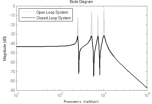Figure 18. Bode diagram of closed-loop system and open-loop system

Comparison of the impulse response of the closed-loop system with this controller and the impulse response of the open-loop system (Figure 19) shows the performance of the controller. This controller suppresses all vibration in less than 0.4 seconds.

Figure 19. Impulse response of the open-loop and closed-loop system

Actuator voltage of this controller during the impulse response is plotted in Figure 20.

Figure 20. Input control for impulse response of the closed-loop system

As one can see, the maximum amplitude of the actuator voltage is under about 100 Volts.

Also, the open-loop and closed-loop responses to a random disturbance in duration of 10 seconds are compared in the Figure 21. Actuator voltage is shown in Figure 22, too.

Figure 21. Closed-loop system and open-loop system responses to a random disturbance

Figure 22. Control input of closed-loop system in duration of a random disturbance

The designed controller was mounted on the nominal plant. For investigation of the robust performance of the uncertain closed-loop system with the designed controller by structured singular value analysis Figure 23 is obtained. This plot shows upper/lower bounds of uncertain closed-loop structured singular values in frequency domain.

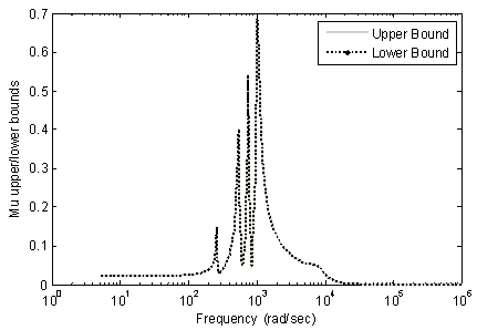Figure 23. µ bounds of uncertain closed-loop system

The performance margin is the reciprocal of the structured singular value and if the magnitude of the structured singular value were under unit, in all frequency range, the system has robust performance. Therefore, upper bounds from structured singular value become lower bounds on the performance margin and critical frequency associated with the upper bound of the structured singular value, here is. In addition, the system can tolerate up to 146% of the modelled uncertainty without losing of desired performance. Note that robust performance guarantees robust stability of the uncertain system.

4.3. A Comparison between Two Approaches

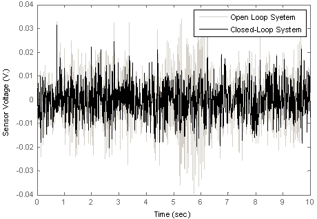
Consider again step response of each designed controller. As one can see, designed controller using µ synthesis suppresses the structure vibration in a less time than one designed by LMI approach. Instead, actuator voltage in the first one is more than the second, so more powerful actuator is needed in the controller that designed by µ synthesis approach. Comparison of bode diagram of these two controller confirms this claim. µ bounds of two closed-loop systems are nearly similar. Therefore, two closed-loop systems can tolerate equal modelled uncertainty without losing of desired performance.

However, most different between two closed-loop systems is in their response to equal random disturbances. As one can see in Figure 15 and figure 21, the performance of the LMI-based designed controller in suppression of a Gaussian random disturbance is better than one obtained by µ synthesis. Figure 24 shows this fact more clear.

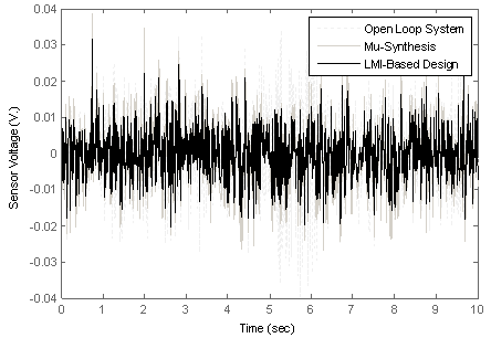Figure 24. Closed-loop with µ-synthesis and LMI-based design systems and open-loop system responses to a random disturbance

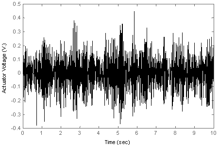
The most attractive phenomena are resulted by comparison of the actuator voltage of two systems during random disturbance applying. As one can see in Figure 16 and Figure 22, the actuator voltage of LMI-based controller is less than another one.

Obtained results shows that the controller designed using LMI approach is more convenient two suppress the random vibration of a smart structure. And this because of minimizing the closed-loop norm from disturbance to system output in LMI approach while in µ synthesis approach the closed-loop norm from disturbance to system output is minimized.

5. Conclusions

Vibration control of a simply supported, thin plate with collocated piezoelectric actuator and sensor as a general smart structure has been achieved using two different approaches of robust controller designing. In the first designing, µ synthesis approach was used. In this method an optimal robust is obtained to minimize norm from disturbance input to desired output (sensor voltage and actuator voltage). LMI-based controller design is used as second method. In this approach norm is used for obtaining appropriate robustness against truncated modes, whereas norm responsible is to obtain a good performance.

Obtained results show that performance and robustness of two designed controllers are the same in the frequency domain and impulse response. However, obtained performances of two designed controllers are different under a random Gaussian disturbance. Moreover, the LMI-based controller response is obviously better than that designed by µ synthesis approach. These results show the ability of the norm designing in rejection of random disturbances.

Future works will be focused on two branches, first implementing these control approaches on real smart structures, experimentally. Next, by using other control approaches vibration suppression and structural acoustic active control can be investigated.