Mohamed B. El Mashade
Electrical Engineering Dept., Faculty of Engineering, Al Azhar University, Nasr City, Cairo, Egypt
Correspondence to: Mohamed B. El Mashade, Electrical Engineering Dept., Faculty of Engineering, Al Azhar University, Nasr City, Cairo, Egypt.
| Email: |  |
Copyright © 2012 Scientific & Academic Publishing. All Rights Reserved.
Abstract
Our scope in this paper is to treat the problem of detecting what is called moderately fluctuating targets when the operating environment is contaminated with a number of outlying targets along with the target under test (multiple-target situations). The illumination of this important class of radar targets by a coherent pulse train, return a train of correlated pulses with a correlation coefficient in the range 0<ρ<1 (intermediate between SWII & SWI). To achieve this goal, we choose the OS based type of adaptive detectors owing to its immunity to interfering targets. However, the homogeneous performance of OS technique is always lower than that of the CA scheme. Therefore, it is preferable to choose the more efficient version, which combines the benefits of these two schemes, of the adaptive detectors. This modified version is known as censored mean-level (CML) in the literature. It implements trimmed averaging of a weighted ordered range samples. Here, the detection performance of the CML processor is analyzed on the assumption that the radar receiver collects data from M successive pulses and the radar system operates in target multiplicity environments. The primary as well as the secondary interfering targets fluctuates in accordance with χ2 fluctuation model. SWI and SWII cases represent the situations where the signal is completely correlated and completely decorrelated, respectively, from pulse to pulse. Exact expressions are derived for the detection and false alarm rate performances in nonideal situations. For weak SNR, it is shown that the processor performance improves as the correlation coefficient ρ increases and this occurs either in the absence or in the presence of outlying targets. This behavior is rapidly changed as the SNR becomes stronger where the processor performance degrades as ρ increases, and the SWII and SWI models embrace all the correlated target cases.
Keywords:
Adaptive Radar Detectors, Postdetection Integration, Partially-Correlated Χ2 Fluctuating Targets, Swerling I and II Models, Target Multiplicity Environments
Cite this paper:
Mohamed B. El Mashade, "Target-Multiplicity Analysis of CML Processor for Partially-Correlated χ2 Targets", International Journal of Aerospace Sciences, Vol. 1 No. 5, 2012, pp. 92-106. doi: 10.5923/j.aerospace.20120105.02.
1. Introduction
Radar target characteristics are the driving force in design and performance analysis of all radar systems. Although the Swerling models for target fluctuation specifications together with the nonfluctuating case bracket the behavior of fluctuating targets of practical interest, they still inadequate as description models for the fluctuation behavior of all target populations of importance. On the other hand, most radar echoes result from the coherent combination of the contributions of many scaterers such as in the cases of clutter (e.g. rain) and of the hot spots of an aircraft. For such echoes, a convenient coherent model is a wide sense stationary Gaussian process with an assigned autocorrelation function. Such targets are termed as moderately fluctuating. The Swerling I and II (SWI & SWII) models are regarded as limiting cases relevant to a flat autocorrelation function (SWI case) or to a Dirac impulse case (SWII model). The detection of this type of radar target fluctuations is of great importance[1-3]. In modern radar systems, equipped with automatic detection circuits, the use of constant false alarm rate (CFAR) algorithms is necessary to keep false alarms at a suitably low rate in an a priori unknown, time varying and spatially non-homogeneous environment. A variety of CFAR techniques are developed according to the logic used to estimate the unknown noise power level. An attractive class of such schemes includes cell-averaging (CA), ordered - statistics (OS) and their modified versions. The threshold in a CFAR detector is set on a cell basis using estimated noise power by processing a group of reference cells surrounding the cell under test. The CA processor is an adaptive scheme that can play an effective part in much noise and clutter environments, and provide nearly the best ability of signal detection while reserving the enough constant false alarm rate. This algorithm has the best performance in homogeneous background since it uses the maximum likelihood estimate of the noise power to set the adaptive threshold. However, the existence of heterogeneities in practical operating environments renders this processor ineffective[3]. Heterogeneities arise due to the presence of multiple targets and clutter edges. In the case of multiple targets, the detection probability of CA degrades seriously due to the non-avoidance of including the interfering signal power in noise level estimate. Consequently, this in turn leads to an unnecessary increase in overall threshold. When a clutter edge is present in the reference window and the test cell contains a clutter sample, a significant increase in the false alarm rate results. Both of these effects worsen as the clutter power increases. In order to overcome the problems associated with non-homogeneous noise backgrounds, alternative schemes have been developed to address this issue, including OS and its versions as well as various windowing techniques aimed to exclude heterogeneous regions. The well-known OS processor estimates the noise power simply by selecting the Kth largest cell in the reference set of size N. It suffers only minor degradation in detection probability and can resolves closely spaced targets effectively for K different from the maximum. However, this processor is unable to prevent excessive false alarm rate at clutter edges, unless K is very close to N, but in this case the processor suffers greater loss of detection performance[4]. In this situation, the censored mean-level (CML) scheme, in which a few of the largest reference cells are excised, is suggested[5]. The performance of this detector is quite robust in the presence of extraneous targets as long as their number is less than or equal to the number of the censored cells from the reference channel[6-8]Following this introduction, we review the detection performance of the CML in a locally homogeneous noise environment and extend the results to the multiple-target situation, where the moderately fluctuating model is used to represent the primary as well as the secondary interfering targets. Once the problem under consideration is formulated in section II, we proceed to consider the performance of the CML in section III. The key step in our analysis is the evaluation of the moment generating function (MGF) of the noise level estimate. We are able to calculate this MGF analytically for the case where the reference channel is free of or contaminated with a specified number of outliers. Section IV is devoted to our numerical results and we terminate this research by a brief discussion about the obtained results along with our conclusions.
2. Theoretical Background and Problem Formulation
The block diagram of typical CFAR with post-detection integration of M pulses is shown in Figure (1). Here, we consider a radar system in which time diversity transmission is employed and assume that M pulses hit the target. Since the signal-to-noise ratio (SNR) is a popular measure of effectiveness of a radar receiving system for combating noise, the maximization of this parameter is one of the earliest criteria investigated. In the early days of the receiver art, band pass filtering techniques were developed to effect discrimination between a desired signal and an interfering signal with adjacent but non-overlapping spectra. A filter that maximizes SNR may be regarded as an extension of this concept. Matched filter theory is one of the important results of this criterion. Therefore, the received IF signal is applied to a matched filter, the output of which is then passed through a square-law device to extract the baseband signal. This signal is then sampled and the sampling rate is chosen in such a way that the samples are statistically independent. The square-law detected video range samples are sent serially into a shift register of N+1 resolution cells resulting in a matrix of Mx(N+1) observations which are denoted by yij. The M observations from the cell under test, which is the one in the middle of the processing window, are represented by y0. The center bin (test cell) is tested on whether it contains a target’s return or not. The detection procedure involves the comparison of the received signal with a certain threshold. The CFAR schemes set this threshold adaptively according to local information on the background noise power. The estimation of the mean power of the local clutter (Z) is usually based on the N neighboring bins. The name of the specific CFAR detector is determined according to the kind of operation used to estimate this unknown power. In this manuscript, we are concerned with the censored mean-level (CML) processor which is hybrid between CA and OS schemes.In order to analyze the detection performance of the underlined processor, let the input to the square-law device consists of M-pulses, each composed of a steady signal component and Gaussian noise. Denote the in-phase and quadrature components of the signal over the M-pulses by the Mx1 vectors Si and Sq, respectively, and denote the corresponding components of the noise by Mx1 vectors Ni and Nq. Then, the integrated output of the square-law device takes a form given by | (1) |
The moment generating function (MGF) associated with the random variable (RV) y0 is defined as | (2) |
In the above expression, ω represents the variable corresponding to the transformed observation space, ƒy(.) denotes the probability density function (PDF) of the RV y0. The substitution of Eq.(1) in Eq.(2) yields | (3) |
If Ni and Nq are independent and identically distributed (IID) Gaussian random vectors, one may write | (4) |
By substituting Eq.(4) into Eq.(3), one obtains | (5) |
Completing the squares in Ni and Nq and integrating over Ni and Nq gives | (6) |
If the signal component fluctuates, then the MGF of the square-law detector is a weighted average, accounting for the PDF of the in-phase and quadrature components of the signal. Hence, for a fluctuating target, the MGF of the detector output is[12]  | (7) |
Assuming that Si and Sq are IID with PDF ƒS(s), we have  | (8) |
2.1. Correlated χ2 Signal Model
Most radar targets are complex objects and produce a wide variety of reflections. These targets often require different models to characterize the varied statistical nature of their responses. A radar target whose return varies up and down in amplitude as a function of time is known as fluctuating target. The fluctuation rate may vary from essentially independent return amplitudes from pulse-to-pulse to significant variation only on a scan-to-scan basis. The χ2 family is one of the most radar cross section fluctuation models. The distribution of this χ2 with 2ҝ degrees of freedom has a PDF of the form[11] | (9) |
where  is the average cross section over all target fluctuations and U(.) denotes the unit step function. When ҝ=1, the PDF of Eq.(9) reduces to the exponential or Rayleigh power distribution that applies to the Swerling cases I and II.It is of great importance to note that the above expression represents the PDF of the sum of the squares of 2ҝ real Gaussian random variables or the sum of the squared magnitudes of ҝ complex Gaussian random variables. Therefore, if ҝ=1, then σ may be generated as σ= x12 + x22, where xi’s are IID Gaussian random variables, each with zero mean and
  /2 variance. Thus, if α=
  /2, we can write the PDF of the magnitude of the in-phase component u (u=x1) as
 | (10) |
To accommodate an Mx1 vector of correlated χ2 RV’s with two degrees of freedom, we introduce the PDF of the M-dimensional vector X1 | (11) |
In the above expression, Λ represents the correlation matrix of x11, x12, ……, x1M, and T denotes the vector transpose. The substitution of Eq.(11) into Eq.(8) yields | (12) |
The symbol I represents the identity matrix. Carrying the above integration leads to | (13) |
Expressing the determinant of Λ in terms of the nonnegative eigenvalues λi’s, i=1, 2, …., M, Eq.(13) takes the form | (14) |
ψ=2σ2 represents the noise power and A=2α/ψ denotes the average SNR. It is of importance to note that the effective fluctuation statistics of the signal to be detected is completely determined by the eigenvalues of the matrix Λ. For example, if the signal to be detected has an effective Swerling II fluctuation statistics, then all eigenvalues of Λ are equal. Swerling I fluctuation model, on the other hand, results effectively when all eigenvalues except one are equal to zero. Eigenvalue distributions between these two limiting cases correspond to fluctuation statistics that lie between SWII and SWI models. In other words, λ1=M, λi=0 for 2 ≤ i ≤ M, for slow fluctuation (SWI), while λi=1 for 1 ≤ i ≤ M, for fast fluctuation (SWII). Therefore, for these distinct models, Eq.(14) has a form given by | (15) |
In view of Eq.(14), the solution for the partially correlated case requires computation of the eigenvalues of the correlation matrix Λ. It is assumed here that the signal has a stationary statistics and it can be represented by a first order Markov process. These assumptions result in a Toeplitz nonnegative definite matrix of the following general form: | (16) |
Eqs.(14-16) are the basic formulas of our analysis in this manuscript.The PDF of the output of the ith test tap is given by the Laplace inverse of Eq.(14) after making some minor modifications. If the ith test tap contains noise alone, we let A=0, that is the average noise power at the receiver input is ψ. If the ith range cell contains a return from the primary target, it rests as it is without any modifications, where A represents the strength of the target return at the receiver input. On the other hand, if the ith test observation is corrupted by an interfering target return, A is replaced by I, where I denotes the interference-to-noise ratio (INR) at the receiver input.
3. Processor Performance Analysis
The CML detector has been introduced to alleviate the problem of extraneous target returns and the degradation caused by them on the processor performance. This is achieved by excluding a specified number of the largest range-cell variates from the noise level estimate. To analyze this detector, we consider the situation where the reference channel contains R extraneous target returns, each with a power level ψ(1+I), and the remaining N-R cells having thermal noise only with power level ψ. The Lth ordered sample has a cumulative distribution function (CDF) given by[9] | (17) |
The CDF of the reference cell that contains an extraneous target return can be obtained from | (18) |
where L-1 denotes the Laplace inverse operator and | (19) |
On the other hand, if the reference sample has thermal noise only, its CDF has the same form as that given by Eq.(18) after setting I tends to zero. Thus, | (20) |
To evaluate the processor detection performance, it is necessary to calculate the Laplace transformation of Eq.(17), where it represents the backbone of the determination of the false alarm and detection probabilities. The ω-domain representation of Eq.(17) can be analytically calculated and final expression is given by[12] | (21) |
where  | (22) |
Eq.(21) is the fundamental relation of our analysis. Let us now go to analyze the detector under investigation. The noise characteristics of this detector are estimated through the formula | (23) |
where  | (24) |
are the order statistics of the samples y1, y2, …………., yN. ξ >0 denotes some constant required to achieve an unbiased minimum variance estimate (UMVE) for the noise power. The order statistics y(i)'s, i=1,….., N, are neither independent nor identically distributed RV's even if the original samples yi's, i=1,……, N, are IID random variables. However, when the observations yi's are exponentially distributed, these samples can be written in terms of independent RV's qi's, i=1, ……., L. The relation between the two sets of samples takes the form[7] | (25) |
In terms of the MGF's of y(i)'s, we can compute the MGF's of qi's according to the following relation | (26) |
On the other hand, the above formula can be written in terms of the Laplace transformation of the CDF of the order statistics y(i)'s as | (27) |
As a function of qi's, the noise power level estimate Z(N, L), Eq.(23), becomes  | (28) |
Since the RV's qi's are statistically independent, the MGF of the noise level estimate Z(N,L) can be easily calculated and the result has a mathematical form given by | (29) |
Owing to the large processing time taken by the OS technique in scoring the candidates of the reference set, its practical applications are limited. Employing two simultaneously specialized processors, one for each subset of neighboring cells, it is possible to reduce by half the single set processing time without altering the estimation of the clutter statistics. As a result of this proposal, double-window processors are preferred from the practical application point of view. The reference set is divided into two subsets, of equally size, and the cells of each subset are independently sorting for its noise level to be estimated through a mathematical relation similar to that given in Eq.(23). The leading Zℓ and trailing Zt noise level estimates are combined through the mean operation to obtain the final noise level estimate Zf. Therefore, | (30) |
For simplicity, we take N1=N2=N/2, and 1≤ Li ≤ Ni, i=1, 2. Because of the averaging of the local estimates of the noise power levels, the final noise level estimate has a MGF given by the product of the corresponding MGF's of the leading and trailing noise level estimates. Thus, | (31) |
where | (32) |
In this case, we assume that there are R1 and R2 reference cells amongst the candidates of the leading and trailing subsets that are contaminated by interfering target returns and N1-R1 & N2-R2 contain thermal noise only. Once the MGF of the final noise power level estimate is obtained, the processor detection performance can be easily evaluated. The detection probability is given by[10] | (33) |
In the above expression, T denotes a constant scale factor required to achieve the desired rate of false alarm and A is as previously defined in Eq.(14). The cell under test y0 has a PDF given by | (34) |
with | (35) |
Let us now go to present some of numerical results to test the validity of our derived formulas and to discuss the role that each parameter can play in the behavior of the detection scheme against different operating conditions.
4. Performance Evaluation Results
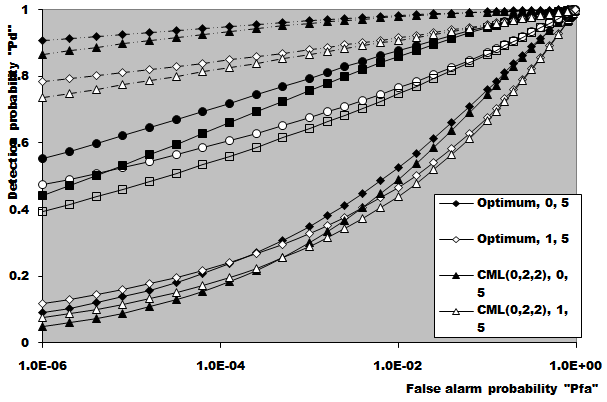
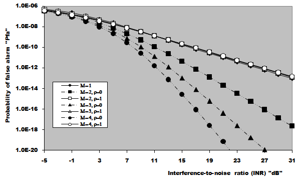
In this section, we apply the exact detection probability determined in the previous section to the performance evaluation of the ML-CML processor Some numerical results, expressed in terms of the variation of the thresolding constant with the false alarm probability, the receiver operating characteristics (ROC's), the detection probability as a function of the primary target SNR, the false alarm probability as a function of the INR of the spurious targets, and the required SNR to achieve a predefined operating point (Pfa, Pd), will be illustrated in this section. We will denote the double-window CML scheme in our results by ML-CML(Nℓ, Nu, ξ), where Nℓ and Nu represent the number of samples that are trimmed from the lower and the upper ends of the reference subset before adding the remainder ones to estimate the unknown noise power level. It is of importance to note that the results displayed here are obtained for a possible practical application of similar parameter values for the two reference subsets as well as equal strengths of the primary and the secondary interfering target returns (SNR=INR). The size of the reference set is chosen to be N=24 and the design false alarm rate is assumed to be Pfa= 10-6. In addition, two upper ordered cells are censored from the elements of the leading and trailing subsets (Nu=2) without any one excised from the lower ends (Nℓ=0). Therefore, the resulting procedure will be denoted as ML-CML(0,2,2) throughout this section. Figure (2) shows the variation of the constant scale factor T with the false alarm rate for different numbers of integrated pulses. It is shown that T decreases as either M or Pfa increases. For comparison, the figure incorporates the variation of the threshold (Topt) of the optimum detector under the same parameter values. It is noted that Topt increases as M increases and decreases as Pfa increases. For a constant rate of false alarm, the fixed threshold Topt must be increased as the number of integrated pulses increases since the received signal becomes stronger with increasing M. In the case of adaptive detection, on the other hand, the thresholding constant T decreases with M for the resultant multiplication of it and the noise power estimate, which increases with M, to be held unchanged in order to keep the rate of false alarm constant. Let us now turn our attention to another type of characteristics which is known in the literature as ROC's. It represents the variation of the detection probability with the false alarm rate at fixed values of SNR of the target under test. Figure (3) shows this variation for SNR of 5, 10, and 15 dB when there are two fully correlated (ρs=1) or fully de-correlated (ρs=0) consecutive sweeps (M=2). The same results for the optimum detector are also included in this figure for the purpose of comparison. An indication (optimum, 1, 5) on a specified curve means that it is drawn for optimum detector when the consecutive sweeps are fully correlated and the strength of the primary target signal return is 5dB. For low SNR, we note that the processor performance for ρs=1 is higher than its performance for ρs=0 when the false alarm rate is low and this behavior is rapidly altered as the false alarm rate increases. This behavior is common for the optimum and the adaptive processors. As the SNR increases, this behavior is not noted and the processor performance for ρs=0 exceeds its performance against ρs=1 case irrespective to the required rate of false alarm. For low values of Pfa, there is a noticeable distinction between the performance of the optimum detector and that of the processor under consideration and their performances approach each other as the rate of false alarm increases. As a final remark, the difference between the two performances, at low rate of false alarm, decreases as the signal returned from the primary target becomes stronger (higher SNR). The third category of performances that measure the ability of the proposed scheme to detect a target in nonideal operating conditions is the detection performance which displays the detection probability as a function the SNR of the target under test when the radar receiver integrates a number of consecutive sweeps. Figs.(4-5) depict the detection performance of the processor under investigation when the operating environment is either homogeneous (R1=R2=0) or multi-target (R1=R2=2) for M=2 and 4, respectively. The candidates of these figures are parametric in the degree of correlation between the target returns and the number of extraneous target returns in each reference subset. In other words, the label ρ=0.5, (2, 2) on a specified curve means that it is plotted for a 50% degree of correlation and in the presence of two interfering target returns amongst the contents of each reference subset (R1=2 & R2=2). From the results of these two figures, it is noted that the processor performance improves as either the number of integrated pulses increases or the degree of correlation between the target returns decreases. In addition, the difference between the processor performance in the absence (homogeneous) and in the presence (multi-target) of outlying targets is not large, given that the number of these interferers is within its allowable range (R ≤ Nu). Moreover, the two performances tend to be the same as the SNR becomes higher. It is of importance to note that the results presented in these two figures are calculated for a possible practical application of equal strengths as well as equal degrees of correlation for the primary and the secondary interfering targets (INR=SNR, ρi=ρs). Our attention is still concerned with multiple-target situation, where the non-homogeneous ROC's of the detector under investigation is displayed in Figure (6) when two cells amongst the samples of each reference subset are contaminated with spurious target returns (R1=R2=2). Since SWII and SWI fluctuating target models represent the boundary limits for the degree of correlation, we are interested in this figure with these two models for the primary and the secondary interfering targets, where SWII represents zero degree of correlation while SWI model denotes the case of 100% correlation. The curves of this family are labeled according to the model of the primary target, the model of the outlying target, and the intensity of the returned signal. On the other hand, an indication (SWII, SWI, 10) on a curve means that its results are evaluated for the case where the primary target follows SWII in its fluctuation, the extraneous target's fluctuation is of SWI model, and for INR=SNR=10dB. Since we have two fluctuation models, there are four possible combinations: (SWII, SWII), (SWI, SWI), (SWII, SWI), and (SWI, SWII). For each combination, the signal strength is allowed to be varied from 5dB to 15dB with a step of 5dB. For low SNR, we show that the processor performance when the primary target fluctuation follows SWI is higher than its performance when the primary target fluctuates in accordance with SWII given that the false alarm rate is held constant at low value. For higher values of false alarm rate, the processor behavior is reversed; the primary target fluctuation model of SWII gives higher performance than the case where it fluctuates following SWI model. In each one of these cases, the processor performance when the secondary interfering target fluctuates in accordance with SWI is higher than its performance for the case where the fluctuation of the outlying target follows SWII model. As the signal strength becomes stronger, the processor performance attains its highest values for the (SWII, SWI) combination after which the (SWII, SWII) combination comes, the (SWI, SWI) combination, and the worst performance is obtained when the primary and the secondary interfering targets fluctuate in accordance with SWI and SWII models, respectively. To confirm this conclusion, Figure (7) shows the target multiplicity detection performance of the ML-CML(0, 2, 2) scheme for different fluctuation models for the primary and the secondary extraneous targets when the radar receiver incorporates a video integrator amongst its basic elements where it integrates 2, 3, and 4 pulses. The curves of this figure are parametric in the number of integrated pulses, fluctuation model of the primary target, and fluctuation model of the outlying target. In other words, M=3, (SWI, SWII) on a given curve means that it is drawn when the primary target fluctuates following SWI model, the secondary target fluctuates according to SWII model and the data of processing are taken from three consecutive sweeps (M=3). The processor detection performance for the case where the fluctuation models of the primary and the secondary interfering targets are SWII and SWII, respectively, is higher than that for the case where these models are SWI and SWII, respectively. As M increases, there is an improvement in the processor performance in any case. As a reference, this figure contains the single sweep curve (M=1) to show to what extent the processor performance may improve as the number of integrated pulses increases. To illustrate the effect of the number of interfering target returns on the processor performance, Figure (8) depicts the same detection performance of the scheme under consideration, as in Figure (7), except that the number of outlying target returns is greater than their allowable range (Nu=2). Note that the full scale of this figure is 80% instead of 100% in the normal state. The candidates of this figure are labeled in the correlation coefficient between the primary target returns (ρ1), the correlation coefficient between the interfering target returns (ρ2), and the number of integrated pulses (M). ρi=0, i=1 & 2, means that SWII fluctuation model is proposed for the underlined target, while ρi=1, i=1 & 2, indicates that the target under investigation fluctuates in accordance with SWI model. From the displayed results, it is noted that there is a noticeable degradation in the processor performance along with all the previous conclusions are also noticed in this figure. Let us now turn our attention to the processor false alarm rate performance and the effect of the interfering targets on keeping it constant or decayed as the strength of the interference becomes stronger. Figure (9) shows this performance, in multiple-target situation, when there are two interfering target returns amongst the contents of each reference subset (R1=R2=2) and these targets fluctuate following SWI and SWII models. For low interference level, SWI fluctuation model tends to give false alarm rate performance which is higher than that obtained by SWII model and as the interference level becomes stronger, the two performances tend to be the same. Higher false alarm rate performance means that the false alarm probability approaches its design value which is 10-6 in the present case. As M increases, there is an improvement in the processor false alarm rate performance. For the purpose of comparison, the single sweep false alarm rate performance is also included in this figure. To show the effect of increasing the number of interfering targets on the false alarm rate of the processor under test, we retrace the results of Figure (9) under the same operating conditions except that the number of outlying target returns is chosen to be out of its allowable range. Figure (10) illustrates the M-sweeps variation of the actual false alarm rate with the strength of the interference level for R1=R2=3. In this case, the false alarm probability decreases continuously as the intensity of the interference level becomes higher and the SWI (ρ=1) model still gives the best false alarm rate performance. On the other hand, the rate of decreasing for SWII (ρ=0) model is higher than that for SWI model. In addition, the rate of decreasing when the extraneous target fluctuates following SWII increases as M increases, while this rate rest approximately unchanged when the fluctuation of the secondary interfering target follows SWI model. As M increases, the false alarm rate performance degrades for fluctuating targets of SWII model, while it remains approximately unchanged from the single sweep case (M=1) when the spurious targets fluctuate following SWI model.Finally, it is required to evaluate the necessary SNR to achieve a preassigned value for the detection probability given that the false alarm rate is held constant. Figure (11) displays these results for the SNR, required to verify an operating point of (Pfa=10-6, Pd=90%), for two and four integrated pulses, as a function of the correlation coefficient (ρ) between the target returns, when the radar receiver operates in either ideal or multiple-target environment. Identical values are assumed for the primary and the secondary outlying target returns from the signal strength and correlation coefficient points of view. For comparison, the results of the optimum detector along with the processor single pulse required SNR are also included in this figure. The required SNR increases smoothly as ρ increases and the rate of increasing becomes higher as ρ tends to 1. As M increases, the required SNR decreases and their values for homogeneous case (R1=R2=0) are always lower than their corresponding values for multitarget (R1=R2=2) case. In addition, the required SNR values approach their corresponding values for the optimum detector as the number of integrated pulses increases. 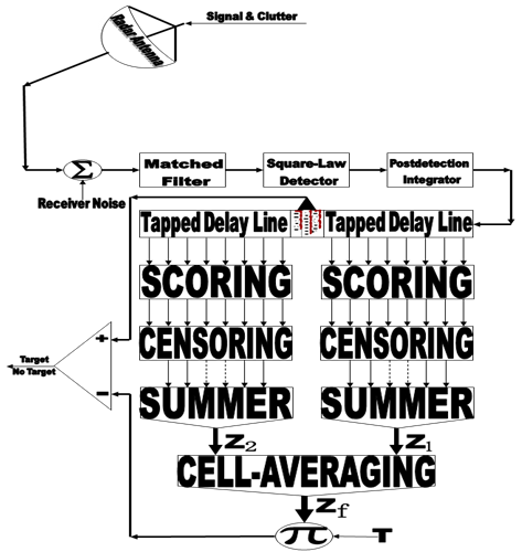 | Figure (1). Architecture of the censored mean-level detector with postdetection integration |
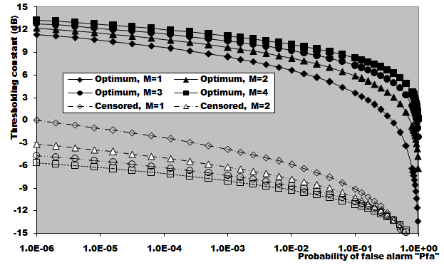 | Figure (2). Thresholding constant (dB) versus false alarm probability of ML-CML(0,2,2) CFAR detector, parametric in M, for a reference window of size 24 cells |
 | Figure (3). Homogeneous ROC of ML-CML(0,2,2) CFAR scheme, for fully correlated and fully decorrelated chi-square fluctuating targets, when N=24, and M=2 |
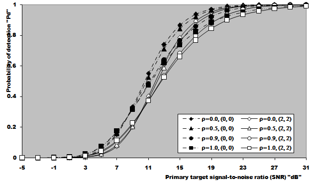 | Figure (4). Partially-correlated chi-square target detection performance of ML-CML(0,2,2) CFAR scheme, in homogeneous and multitarget situations, when N=24, M=2, Pfa=1.0E-6, and R1=R2=2 |
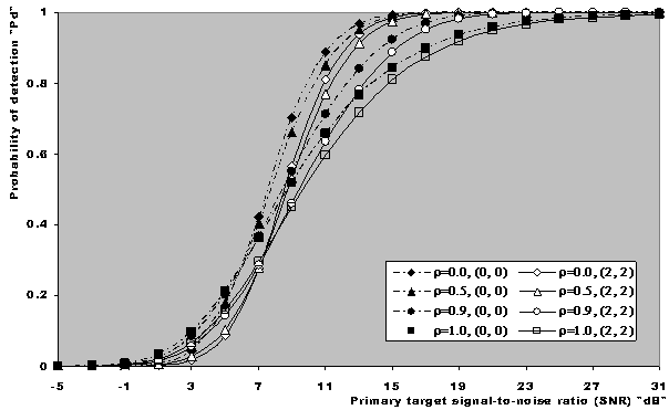 | Figure (5). Partially-correlated chi-square target detection performance of ML-CML(0,2,2) CFAR scheme, in homogeneous and multitarget situations, when N=24, M=4, Pfa=1.0E-6, and R1=R2=2 |
 | Figure (6). Multiple-target ROC of ML-CML(0,2,2) CFAR processor, for fully correlated and fully decorrelated chi-square fluctuating targets, when N=24, M=2, and R1=R2=2 |
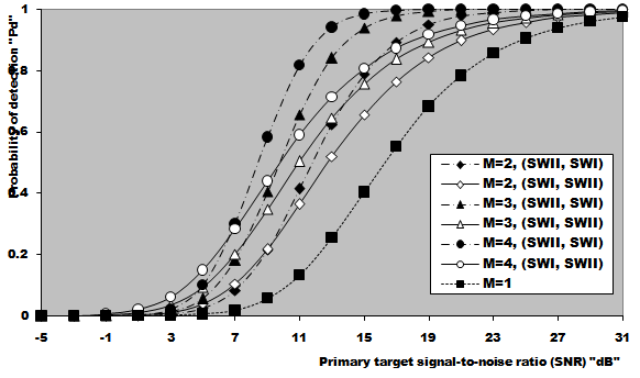 | Figure (7). Target-multiplicity detection performance of ML-CML(0,2,2) CFAR processor, for fully decorrelated and fully correlated targets, when N=24, Pfa=1.0E-6, and R1=R2=2 |
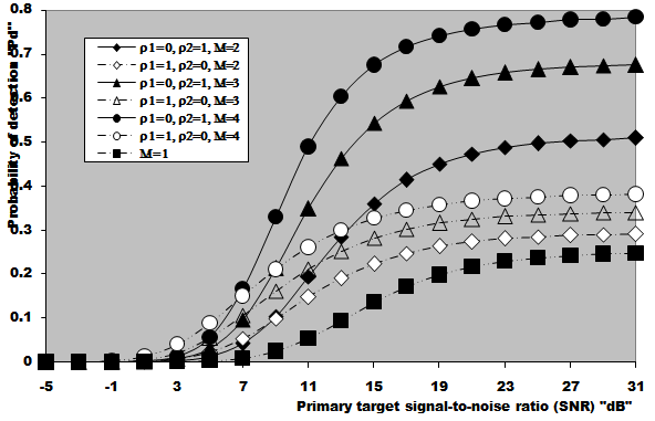 | Figure (8). Target multiplicity detection performance of ML-CML(0,2,2) processor, for fully correlated and fully decorrelated chi-square fluctuating targets, when N=24, Pfa=1.0E-6, and R1=R2=3 |
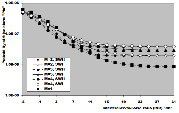 | Figure (9). Actual false alarm probability against interference-to-noise ratio of ML-CML(0,2,2) CFAR processor, for Swerling fluctuating targets, when N=24, design Pfa=1.0E-6, and R1=R2=2 |
 | Figure (10). Actual probability of false alarm versus the strength of interfering targets of ML-CML(0,2,2) CFAR scheme, for fully correlated and fully decorrelated chi-square fluctuating targets, when N=24, design Pfa=1.0E-6, and R1=R2=3 |
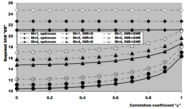 | Figure (11). Required SNR to achieve an operating point (1.0E-6, 0.9) for partially correlated chi-square target detection performance of ML-CML(0,2,2) processor when N=24, and R1=R2=2 |
5. Conclusions
This paper is devoted to the analysis of an adaptive detector which is an alternative to the mean-level processor that achieves robust detection performance in multitarget environment by excising several of the largest samples of the maximum likelihood estimate of the background noise level. An exact analytical expression is derived for the detection probability of the ML-CML scheme in the case where the radar receiver incorporates a video integrator amongst its basic elements and the CFAR circuit processes data that are returned from partially-correlated χ2 targets. The operating environment is treated as either free of outlying targets (homogeneous) or contains some of extraneous targets along with the primary target of interest. The numerical results are obtained for a possible practical application that the signal strength as well as the degree of correlation between successive data for the primary and the secondary interfering targets are assumed to be the same. Special interest is focused to the boundaries of the correlation coefficient which correspond to SWII model for ρ=0 and to SWI model for ρ=1. As predicted, it was found that the processor homogeneous performance when the fluctuation of the primary target follows SWII model is higher than its performance when it fluctuates in accordance with SWI model. In multiple-target situation, on the other hand, the processor performance in the presence of outlying fluctuating targets of SWI model exceeds its performance in the case where the spurious targets fluctuate following SWII model. The final conclusion that can be extracted from our presented data is that the processor performance can be improved by increasing the number of integrated pulses and/or decreasing the degree of correlation between the successive data.
References
| [1] | Rickard, J. T. & Dillard, G. M. (1977), “Adaptive detection algorithm for multiple target situations”, IEEE Transactions on Aerospace and Electronic Systems, AES-13, (July 1977), pp. 338-343. |
| [2] | Ritcey, J. A. (1986), “Performance analysis of the censored mean level detector”, IEEE Transactions on Aerospace and Electronic Systems, AES-22, (July.1986), pp. 443-454. |
| [3] | Aloisio, V. di Vito, A., & Galati, G. (1994), “Optimum detection of moderately fluctuating radar targets”, IEE Proc.-Radar, Sonar Navig., Vol.141, No.3, (June 1994), pp. 164-170. |
| [4] | El Mashade, M. B. (1995), “Detection performance of the trimmed mean CFAR processor with noncoherent integration”, IEE Radar, Sonar Navig., Vol.142, No.1, (Feb. 1995), pp. 18-24. |
| [5] | El Mashade, M. B. (1995), “Analysis of the censored mean level CFAR processor in multiple target and nonuniform clutter”, IEE Radar, Sonar Navig., Vol.142, No.5, (Oct. 1995), pp. 259-266. |
| [6] | El Mashade, M. B. (1996), “Monopulse detection analysis of the trimmed mean level CFAR processor in nonhomogeneous situations”, IEE Radar, Sonar Navig., Vol.143, No.2, (April 1996), pp. 87-94. |
| [7] | El Mashade, M. B. (1998), “Multipulse analysis of the generalized trimmed mean CFAR detector in nonhomogeneous background environments”, AEÜ, Vol.52, No.4, (Aug. 1998), pp. 249-260. |
| [8] | El Mashade, M. B. (1998), “Detection analysis of linearly combined order statistic CFAR algorithms in nonhomogeneous background environments”, Signal Processing “ELSEVIER”, Vol.68, (Aug. 1998), pp. 59-71. |
| [9] | El Mashade, M. B. (2006), "Performance Comparison of a Linearly Combined Ordered-Statistic Detectors under Postdetection Integration and Nonhomogeneous Situations", Journal of Electronics (China), Vol.23, No.5,(September 2006), pp. 698-707 . |
| [10] | El Mashade, M. B. (2008), "Analysis of CFAR detection of Fluctuating Targets",Progress In Electromagnetics Research (PIER) C, Vol. 2, pp. 65-94, 2008. |
| [11] | El Mashade, M. B. (2008), "Performance improvement of adaptive detection of radar target in an interference-saturated environment",Progress In Electromagnetics Research (PIER) M, Vol. 2, pp. 57-92, 2008. |
| [12] | El Mashade, M. B. (2008), "Performance analysis of OS structure of CFAR detectors in fluctuating target environments",Progress In Electromagnetics Research (PIER) C, Vol. 2, pp. 127-158, 2008. |
 Abstract
 Reference
 Full-Text PDF
 Full-Text HTML