Sanjay Jayaram 1, Darren Pais 2
1Aerospace and Mechanical Engineering Department, Saint Louis University, Saint Louis, MO, 63103, USA
2Mechanical and Aerospace Engineering Department, Princeton University, Princeton, NJ 08544, USA
Correspondence to: Darren Pais , Mechanical and Aerospace Engineering Department, Princeton University, Princeton, NJ 08544, USA.
| Email: |  |
Copyright © 2012 Scientific & Academic Publishing. All Rights Reserved.
Abstract
SLUCUBE-2 is a 1U CubeSat with maximum dimensions of 10 x 10 x 10 cm3 and a mass of one kilogram. CubeSat constraints’ poses significant challenges in the design of the attitude control system. As a result, passive attitude stabilization involving gravity-gradient methods, permanent magnet alignment and/or viscous dampers, etc., are frequently considered for such missions. SLUCUBE-2 is stabilized using a passive magnetic attitude stabilization system, based on permanent magnets and an energy dissipation system consisting magnetic hysteresis rods. However, sizing the system parameters, predicting the in-orbit performance and accuracy of passive magnetic stabilization systems is not trivial, challenges being accurate modeling of the hysteresis rods magnetization and the evaluation of the rods magnetic parameters, such as apparent permeability, remanence and coercive force. The research focus in this paper is design and analysis of passive stabilization using nonlinear models of hysteresis behavior and nonlinear model of spacecraft attitude dynamics. Methods and results of Nonlinear and Quaternions-based mathematical model for satellite motion involving permanent magnets and hysteresis effects is presented. This study has resulted in determining the size and the number of the permanent magnets and hysteresis rods required to stabilize the spacecraft.
Keywords:
Picosatellite, Passive Stabilization, Permanent Magnets, Hysteresis Magnetic Material, Dynamic Model-based Simulation
Cite this paper:
Sanjay Jayaram , Darren Pais , "Model-based Simulation of Passive Attitude Control of SLUCUBE-2 Using Nonlinear Hysteresis and Geomagnetic Models", International Journal of Aerospace Sciences, Vol. 1 No. 4, 2012, pp. 77-84. doi: 10.5923/j.aerospace.20120104.04.
1. Introduction
The method of attitude control for LEO satellites must be selected between a completely passive system, or an active control system that produces the desired control torque based on signals indicating deviation from desired attitude, or a combination thereof. In satellite applications, where a high degree of attitude precision is necessary (camera pointing for example), active control techniques must be employed, involving a collection of sensors, actuators and computer processing. However, many satellite applications exist[1, 2, 3, 4] where the attitude restrictions are not as stringent, and the attitude control system plays the functional role of stabilizing the vehicle and achieving desired orientation for tasks such as antenna pointing and communication. In such applications, completely passive attitude stabilization renders itself as the most suitable option, with significant savings in weight, computational power, system complexity, reliability and system longevity. This trade-off becomes extremely critical in small nano- and pico-class satellites where constraints of mass, volume and power are significant. Various forms of passive attitude stabilization exist[6], particularly common of which are gravity-gradient methods, nutation damping and permanent magnet alignment (Figure 1). Many prior spacecraft missions[1, 2, 3] and current pico and nano spacecraft missions have used permanent magnets and hysteresis materials for passive attitude control. Sizing of these attitude control actuators have been primarily based on experience and intuition rather than design based on simulation and analysis using nonlinear models of hysteresis damping and geo-magnetic field. Passive magnetic attitude control design and analysis for small and pico satellites are becoming more prominent in recent years, specifically for university space missions[12 - 17]. The main contributions of this paper are as follows:• Development of non-linear attitude dynamic equations for CubeSat class spacecrafts.• Design of passive magnetic attitude control and hysteresis damping using nonlinear dynamic models for magnetic hysteresis and earth’s geomagnetic fields, thereby providing a complete dynamic description of passive magnetic attitude stabilization.• Verification of the design using model-based simulation to estimate the number and volume of permanent magnets and hysteresis material required for passive attitude control.• Using Quaternion-based simulation to eliminate singularity conditions.The simulation study presented in the paper shows that the permanent magnet-based satellite stabilization presents significant savings of mass and complexity when compared to active methods, and even relative to other passive techniques such as gravity-gradient stabilization.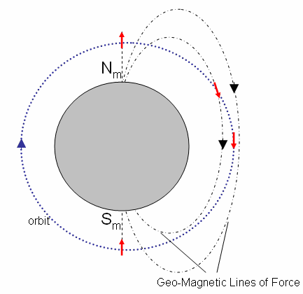 | Figure 1. An illustration of the Earth’s magnetic lines of force. Nm and Sm indicate the magnetic north and south poles respectively and the red arrows illustrate a permanent magnet aligning with the geomagnetic lines of force, along a circular orbit |
2. Cubesat Standard
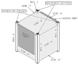 | Figure 2. CUBESAT Standard |
CubeSats are standard pico-satellites created by a joint venture between the California Polytechnic State University San Luis Obispo and Stanford University's Space Systems Development Laboratory. The purpose of the program is to provide uniform standards for nano-satellite design. The fundamental defining feature of the CubeSat standard is its dimensions specifying that the satellite must have the geometry of 10x10x10 cm3 with a mass of no more than 1kg and that the center of gravity must be within 2cm of the geometrical center. Figure 2 shows the CUBESAT standard[ 5].
3. Attitude Dynamics
In this section, dynamic equations of motion necessary to model the orbital motion and attitude of a spacecraft are developed. Numerical solutions to the differential equations presented here provide the time dependent angular velocities and attitude parameters (such as roll, pitch and yaw) with respect to the IRF or the MRF (Figure 3 and 4). The Euler’s equations are initially derived, followed by angular velocity conversions and attitude dynamics equations. To represent transformation from MRF to BRF, a 3x3  transformation matrix
  is presented as shown in Eq. (1).
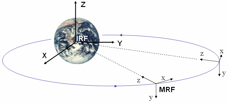 | Figure 3. Reference Frames. IRF is the Earth centered Inertial Reference Frame denoted by XYZ and MRF is the orbit referenced Moving Reference Frame denoted by xyz |
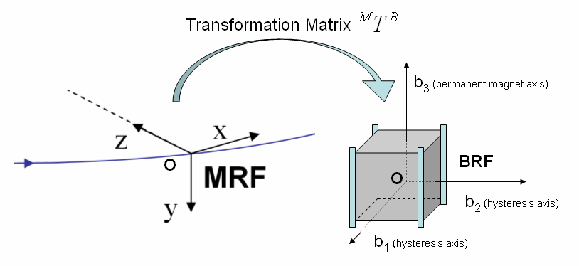 | Figure 4. Relationship between MRF and BRF for a satellite via the  transformation, showing body axes that correspond to permanent magnet and hysteresis material dipole alignment transformation, showing body axes that correspond to permanent magnet and hysteresis material dipole alignment |
 | (1) |
3.1. Euler’s Moment Equation
For an arbitrary time dependent vector  represented in two frames as
  (inertial frame) and
  (body frame), where
  represents the angular velocity of the body frame with respect to the inertial frame, the time derivative of the body frame vector is obtained using the transformation matrix
  as shown in Eq. (2).[8]
 | (2) |
From Newton’s second law, the rate of change of angular momentum of a body is equivalent to the external force acting on it, which is represented in Eq. (3), where  is the angular momentum projected in the inertial frame, and
  is the net external moments, also projected in the inertial frame.
  | (3) |
In the body frame, by definition, the angular momentum is given by Eq. (4), where the 3x3 body mass moment of inertial tensor is represented as  ,
,  | (4) |
Making substitutions using Eq. (3) and Eq. (4) in Eq. (2), Euler’s moment equation as expressed in the satellite BRF, is presented in Eq. (5)(note that  ).[8]
).[8]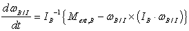 | (5) |
This is the fundamental non-linear equation representing the spacecraft orbital motion in three axes.
3.2. Angular Velocity Conversions, Rotating Frame Angular Velocity
For the orbital motion of the satellite (circular, polar orbit of constant orbital speed), the angular velocity of the MRF with respect to the IRF, as expressed in BRF coordinates using the  transformation matrix is given by Eq. (6), where n is the mean orbital motion of the satellite given by Eq. (7).
 | (6) |
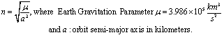 | (7) |
The negative sign in Eq. (6) represents the fact that the orbital angular velocity vector is anti-parallel to the MRF’s y-axis for the orbit. The angular velocity of the BRF with respect to the MRF, can be expressed as, | (8) |
Making a substitution for Eq. (6) into Eq. (8), an expression for the angular velocity of the BRF with respect to the MRF as a function of  is derived,
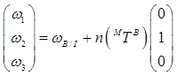 | (9) |
Using the transformation as defined in Eq. (1) in place of , the BRF Euler angle rates obtained from Eq. (9) are as follows: | (10) |
Eq. (5) can be solved numerically to obtain at discrete time-steps. Using Eq. (9), values of ω1, ω2 and ω3 at each time step is computed. Hence, the systems of differential equations in Eq. (5) and Eq. (10) are coupled and are solved simultaneously at discrete time-steps in order to obtain the roll, pitch and yaw angles of the satellite and thereby a description of its attitude. It is also important to note that the systems of equations are non-linear, thereby making it difficult to obtain an analytical solution without very specific constraints. Further, for the system in Eq. (10), it is important to note that there exist singularities for roll angle at . In attitude simulation section (5) of this paper, it will be shown that the roll angle is not critical to the simulation as it rarely approaches 900, thereby validating the choice of
  transformation in Eq. (1). The paper (in section 6) also presents the Quaternion representation of spacecraft attitude that will comprise a linearized representation of Eq. (10) that does not have any singularities.
4. Magnetic and Hysteresis Torque Modeling
The International Geomagnetic Reference Field (IGRF-10) provides a mathematical description of the magnetic field of the Earth. The IGRF expresses the scalar magnetic potential as a series expansion function of distance from the Earth’s center, latitude and longitude. The coefficients of the series expansion are obtained from fitting to satellite measurement data and normalized coefficients associated with Legendre functions. The gradient of the potential function provides the magnetic field lines of force. The DGRF/IGRF website provides a convenient means of obtaining the magnetic field vector in IRF coordinates ( ) with suitable input of latitude, longitude and altitude. While the expressions[9] provide an accurate and widely used technique to compute the geo-magnetic field, the approximate L-Shell model of the magnetic field helps provide a good qualitative description of the field lines[10]. At a given magnetic latitude λ, for a given L-value (measured in Earth Radii, corresponding to a given field line), the field radius R, which is the distance in Earth Radii from an idealized magnetic dipole at the Earth’s center is given by,
 | (11) |
The Cartesian components of R along the X-axis and Z-axis are  and
and  respectively. Using Eq. 11 and plotting the magnetic field in the IRF XZ-plane, a pictorial representation of the geo-magnetic field is obtained, as shown in Figure 5. The two sub-sections to follow this section illustrates the equations that are used to compute permanent magnet torques and hysteresis magnetic torques at a given point in orbit, and a given local magnetic field vector at the point,
  .
.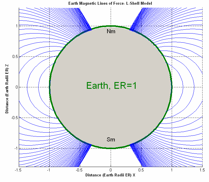 | Figure 5. Earth magnetic field lines using the L-Shell model |
4.1. Permanent Magnet Torque
Assuming perfect dipole distributions of the field around a permanent magnet, the magnetic dipole moment vector  (expressed in the BRF) is computed knowing the magnet’s rated magnetic induction B (Tesla), its volume V (cubic meters), the axis of dipole orientation (positive body b3 axis), and the permeability of free space
  using the expression,[11]
 | (12) |
The geo-magnetic field model described in Eq. (11) provides the magnetic field vector expressed in the IRF,  (Tesla). The external torque exerted by the permanent magnets at a given point in the orbit can now be conveniently computed using a simple cross product as,
 | (13) |
4.2. Hysteresis Damping Torque
Hysteresis magnetic materials are much like permanent magnets in their function, except that these materials are significantly of higher permeability. Under the influence of a changing weak external magnetic field (like the Earth’s field), the hysteresis materials tend to exhibit realignment of dipoles and change in magnetic domain boundaries. These changes result in frictional dissipation of energy at the molecular level, a phenomenon known as hysteresis dissipation. Hysteresis materials have been successfully used for damping satellite oscillations on prior missions. In order to maintain system equilibrium on permanent magnet and field alignment, the hysteresis materials must have their dipole axes orthogonal to the permanent magnets (on the b1 or b2 BRF axes). Hysteresis materials are defined by three key parameters - the saturation induction Bm (Tesla), the remanent induction B0 (Tesla) and the coercivity H0 (Ampere/meter). Using these parameters, the hysteresis loop outer boundaries are modeled as non-linear tangent functions shown in (Eq. (14)) and illustrated in figure 6. Hysteresis damping models used for passive attitude control design for prior missions and many current missions indicate that an approximated linear model of hysteresis behavior is used as shown in figure 7. 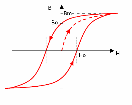 | Figure 6. Variation of magnetic induction (B) with external magnetizing field (H) for a hysteresis material |
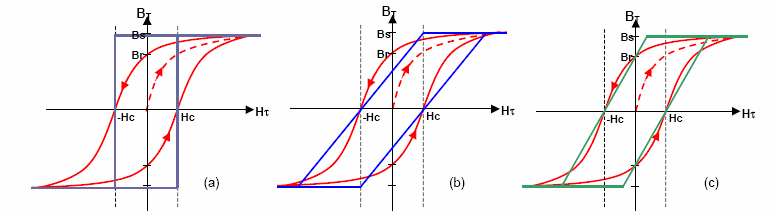 | Figure 7. Approximated Linear Models of Hysteresis Behavior |
 | (14) |
Equation 14 predicts the changing magnetic induction of the hysteresis material (B) dynamically, knowing the component of the external magnetic field (B1, B2 (tesla) → H (Oe, Amperes/m2) along the axis of the hysteresis material, at a certain point and time in orbit. Particularly, changes in the external magnetic field can be related to the magnetic induction of the hysteresis material (and thus the magnetic dipole moment) by the following equation: | (15) |
This dynamic induction can in turn be converted to the corresponding hysteresis damping moments,  using Eqs. (12) (with an x- or y- axis unit vector), and (13), knowing the volume of hysteresis material used or vice versa. Simulations were performed to validate the accuracy of the hysteresis damping model and compared with the experimental investigation from the literature[13]. Figure 8 shows the model-based simulation results and figure 9 shows the experimental results. Comparing the two, it is concluded that the mathematical model accurately represents the results from the experimental investigations.
 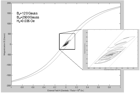 | Figure 8. Model-based Simulation of Hysteresis Loop |
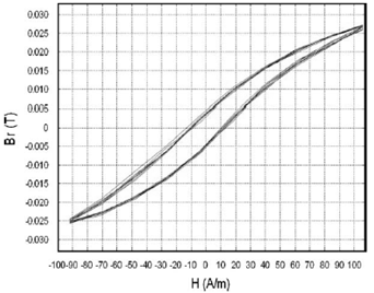 | Figure 9. Experimental Measurement of Hysteresis Loop[ 13] |
5. Attitude Simulation
In this section, using nonlinear dynamic equations developed in previous sections, the state of the system is computed at discrete time steps by numerically solving the systems of differential Eqs. (5) and (10). The state of the system at a given time step can be represented by a single, time-dependent vector comprising the variables in the differential equations as,  . For simulations, it is assumed that the spacecraft is orbiting in a circular, polar orbit in the LEO with an altitude of 800km. The hysteresis material parameters used have the following properties: B0 = 0.012 Tesla, Bm = 0.25 Tesla and H0 = 0.035 Oe. The inertia tensor used for SLUCUBE-2 is,
 | (16) |
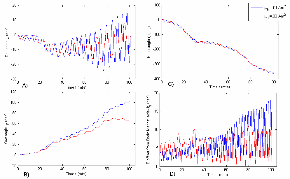
Two scenarios were considered for simulation purposes. In scenario 1, the simulations are performed with all initial conditions in the state vector S(t) (angular velocities and Euler angles) set to zero, and the spacecraft has only permanent magnets for stabilization and no hysteresis dampers. The results of this simulation are presented in figure 8 for one full orbit at different permanent magnet strengths. It should be noted that the higher permanent magnet strength implies a higher frequency of oscillation and higher oscillation amplitude as expected. It should also be noted that the satellite does pitch through the necessary 3600 in one orbit, illustrating that it oscillates about the geo-magnetic field with maximum amplitude of about 200 (figure 10(c) and 10(d)). In scenario 2 (figure 11), simulations were performed introducing the effects of adding hysteresis damping to mitigate the high-amplitude oscillations observed for the higher permanent magnetic dipole stabilization in scenario 1 (figure 10). With the addition of hysteresis damping, the pitch and yaw oscillations are reduced, as well as a reduction in field offset. This is due to the mitigation of oscillations by the hysteresis materials. The hysteresis materials have a lesser long-term effect on mitigating roll oscillations since there are no moments exerted along the roll axis following field alignment (because the hysteresis materials are perpendicular to the alignment axis of the permanent magnets). However, roll oscillation amplitudes are significantly mitigated as seen in figure 11(a).
6. Quaternion Representation
Based on the Euler angle equations presented in Section 2.1, as well as the attitude simulations presented in Section 4, several important drawbacks were noticed. (1) The use of the dynamic simulations in an iterative spacecraft design process requires the initialization of initial conditions, (2) Singularities were occurring at certain angles during the full orbit simulations, and (3) The non-linear nature of the spacecraft dynamics made it inefficient and computationally intensive when computing attitude for a larger number of orbits. To overcome these limitations, a Quaternion-based approach to modeling the attitude of the spacecraft was analyzed and the simulation results are presented in this section.Quaternions are regarded as a 4-tuple of real numbers (i.e. an element of x4) and are typically represented by the letter q, as a combination of a vector in x3 and a scalar (q =  ). Geometrically, Quaternions are related to rotations about a unit vector axis
  by an angle θ using the relationship,
 | (17) |
Details of Quaternion conjugation, multiplication and rotation are presented in various references[7]. Here, only key relationships necessary for modeling the system are presented.For the  transformation, Quaternions are related to Euler angles by the following relationships,
 | (18) |
The rotation matrix is derived from Quaternions using the expression in Eq. (18). 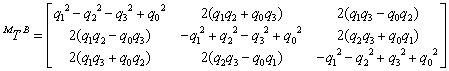 | (19) |
In order to use Quaternions to simulate spacecraft attitude dynamically, a system of differential equations are derived to replace the Euler angle system represented in Eq. (10). These equations are given below: | (20) |
Using Eqs. (5) and (20), and expressing the attitude of the spacecraft in the Quaternion form (Eq. (19)), a convenient model of the spacecraft attitude using Quaternions is derived. These equations are free from singularities and can be simulated for any number of orbits. The system of equations shown in Eq. (20) is linear, hence computationally more efficient. The simulations performed using Quaternion equations are with same initial conditions as that of scenario 1 (figure 10, all initial conditions zero) with the exception that an initial deployment angular velocity of 0.2 rpm is induced along the body b3 (z-axis) to observe the response behavior for undamped oscillation, and further illustrate the mitigation of induced high-amplitude oscillations using hysteresis damping. The results are shown in figure 12, where the dotted blue curve illustrates the magnetic field offset for a zeros initial condition vector, undamped scenario and permanent magnetic dipole strength of 0.03 Am2 (similar to blue curve in figure 10(d)). The green curve represents the addition of a moderate initial deployment spin of 0.2 rpm for the same dipole moment, in undamped conditions. The red curve illustrates the mitigation of the initial permanent magnet axis spin using hysteresis materials of volume 3.75x10⁻⁷ m3.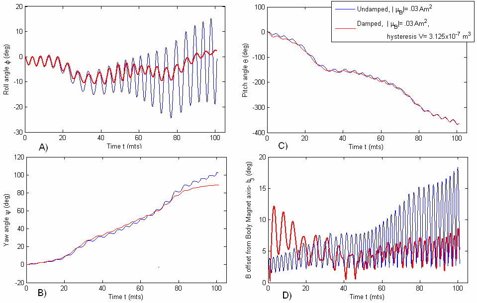 | Figure 10. Scenario 1-Permanent magnet response a) Roll angle response b) Yaw angle response c) Pitch angle response d) B-offset: magnet deviation from field lines, notice higher amplitudes and oscillation frequencies for higher magnetic dipole moment (curves in red). Dipoles: Blue 0.03 Am2, Red: 0.01 Am2 |
 | Figure 11. Scenario 2-Permanent magnet with hysteresis response a) Roll angle response b) Yaw angle response c) Pitch angle response d) B-offset, notice yaw and pitch damping, roll amplitude mitigation (red) |
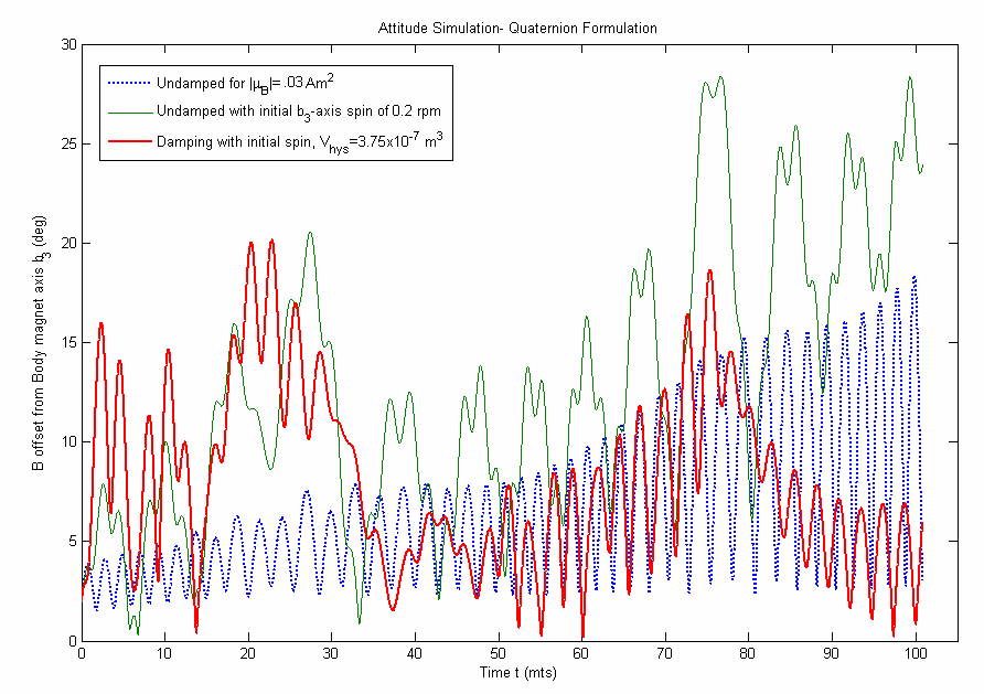 | Figure 12. Attitude Simulation using Quaternion Formulation |
7. Conclusions
The paper has developed and presented an effective method of accurately modeling the earth’s magnetic field using L-shell model and hysteresis damping models. These models have shown to match very closely with the experimental results from existing results. Using these models, the sizing of permanent magnets and hysteresis rods for CubeSat mission is presented. Simulation results indicate that the spacecraft oscillations in orbit can be damped using hysteresis materials, illustrating the effects of adding hysteresis damping to a permanent magnet stabilized system. Quaternion form of the dynamical equations is also presented as an extended study in order to overcome the singularity and complexity disadvantages associated with the Euler angle equations. The results from this paper provides tools necessary for modeling passive magnetically stabilized spacecraft dynamics along with the implementation of these techniques for a specific satellite mission with the results verified through simulations. The final conclusion is that the passive magnetic attitude control is an efficient, reliable and inexpensive technique, particularly suited to the stringent mass, volume, computation and cost restrictive nature of nano and pico-satellite missions.
Appendix A: Nomenclature
 = 3x3 transformation matrix from frame α to frame β
 = roll, pitch and yaw angles respectivelyX, Y, Z = co-ordinate frame representation for the Inertial Reference Frame (IRF)x, y, z = co-ordinate frame representation for the Moving Reference Frame (MRF)
 = co-ordinate frame representation for the Body Reference Frame (BRF)
 = angular velocity of frame α with respect to frame β, expressed in body co-ordinates
 = externally applied (magnetic) moment expressed in body coordinates
 = moment of inertia tensor of the satellite expressed in body coordinates,
  = 3x1 magnetic dipole moment vector
  = external magnetic field vector expressed in frame α
 = Hysteresis material magnetizing fieldB = Hysteresis material magnetic inductionS(t) = state vector for the system at a given time t
 = 4 element (1 scalar and 3 vector) Quaternion representation of attitude
 = Earth’s magnetic field vector in Body Reference Frame
References
| [1] | Kumar, R. R., Mazanek, D. D., and Heck, M. L. (1995), “Simulation and Shuttle Hitchhiker Validation of Passive Satellite Aerostabilization,” AIAA Journal of Spacecraft and Rockets, Vol. 32, No. 5, pp. 806-811. |
| [2] | Whisnant, J. M., Anand, D. K., Psiacane, V. L., and Sturmanis, M. (1961), “Dynamic Modeling of Magnetic Hysteresis,” AIAA Journal of Spacecraft and Rockets, Vol. 7, No. 6, 1970 pp. 697-701. |
| [3] | Fischell R. E., “Magnetic Damping of the Angular Motions of Earth Satellites,” ARS Journal, Vol. 31, No. 9, pp. 1210. |
| [4] | Waydo, S., Henry, D., and Campbell, M. (2002), “CubeSat Design for LEO-Based Earth Science Missions,” IEEE Journal, IEEEAC paper #248, 0-7803-7231-X/01. |
| [5] | Nason, I., Puig-Surai, J., Twiggs, R. (2002), “Development of a Family of Pico-Satellite Deployers based on the CubeSat Standard,” IEEE Journal, 0-7803-7231-X. |
| [6] | Sidi, M. J. (2005), Spacecraft Dynamics and Control, Cambridge, New York. |
| [7] | Kuipers J. B. (1999), Quaternions and Rotation Sequences, Princeton University Press, Princeton NJ. |
| [8] | Pisacane, V. L. (2005), Fundamentals of Space Systems, 2nd ed., Oxford University Press, New York. |
| [9] | Filipski, M. N., Abdullah E. J. (2006), “Nanosatellite Navigation with the WMM2005 Geomagnetic Field Model,” Turkish Journal of Eng. Env. Sci., Vol. 30, pp. 43-55. |
| [10] | Wertz, J. R., Larson, W. J. (1999), Space Mission Analysis and Design, 3rd ed., Microcosm Press, Torrance CA. |
| [11] | Levesque. J. (2003), “Passive Magnetic Attitude Stabilization using Hysteresis Materials,” Universite de Sherbrooke, SIgMA-PU-006-UdeS. URL: http://www.geocities.com/jflev/cubesim.htm |
| [12] | Martinelli, M.I, Sanchez Pena, R.S. (2005), “Passive 3-Axis Attitude Control of MSU-1 Picosatellite”, Acta Astronautica, Vol. 56, pp. 507 – 517. |
| [13] | Santoni, F, Zelli, M. (2009), “Passive Magnetic Attitude Stabilization of the UNISAT-4 Microsatellite”, Acta Astronautica, Vol. 65, pp. 792 – 803. |
| [14] | Gerhardt D. T, Palo E.P (2010) “Passive Magnetic Attitude Control for CubeSat Spacecraft”, 24th Annual AIAA/USU Conference on Small Satellites, Logan, Utah. |
| [15] | Mahmood R, Khurshid K, Zafar A, Islam Q, (2011) “ICUBE-1: First Step towards Developing an Experimental Pico-satellite at Institute of Space Technology”, Journal of Space Technology, Volume 1, No. 1, pp. 5 – 10. |
| [16] | Springmann J.C, Kempke B. P, Cutler J.W, Bahcivan H (2012), “Initial Flight Results of the RAX-2 Satellite”, 26th Annual AIAA/USU Conference on Small Satellites, Logan, Utah. |
| [17] | Shiqiang Z, Xi W, Qian Y (2012), “Integral Design and Analysis of Passive Magnetic Bearing and Active Radial Magnetic Bearing for Agile Satellite Application”, IEEE Transactions on Magnetics, Volume 48, No. 6, pp. 1959 – 1966. |
 Abstract
 Reference
 Full-Text PDF
 Full-Text HTML