1. Introduction

In recent times, particular attention has been directed toward the development of new Global Navigation Satellite Systems (GNSSs), as the European Galileo and the renewed Russian GLONASS. All these systems aim to be interoperable each other and with the GPS, and to be exploited all at once, to provide the user receiver with a large set of measurements, entailing better precision and robustness[1][2].

Software Defined Radio (SDR) is a modern technology that allows to replace part of the hardware of a radio device with a software architecture running on an appropriate digital processor[3][4][5][6]. Such an approach allows the development of reconfigurable terminals, thanks to the ease of access to every single functional block implemented in software. This characteristic happens to be very useful for system designers that are provided with a valuable tool for testing and comparing algorithms and architectures, quickly implemented as simple software modules

In this article we discuss the possibility to implement a SDR receiver capable to jointly process both the GPS and Galileo signals. In particular, we discuss some of the issues that may commonly arise in designing a joint GPS/Galileo software receiver for research purposes, taking as an example our real-time software receiver, N-Gene[7].

Although abundant literature is available on architectures and algorithms for GNSS receivers (see for example[8]—[17] and references therein), it is often difficult and time-consuming to cope with the implementation options arising when passing from the theory to the practice, as itcan be seen even in the recent literature and research activities[15] —[18]. We discuss here implementation choices related to the tracking stage and to the Position-Velocity-Time (PVT) computation, since these are in our opinion the characterizing blocks in a joint GPS/Galileo receiver, when processing measurements from Galileo and GPS at the same time. Since the Galileo signal is not currently available, our tests relied on the signals produced with the Spirent GSS7700 and GSS7800 generators.

The remainder of the paper is structured as follows: in Section II we discuss the architecture of the receiver: subsection A introduces the acquisition stage, while subsections B and C describe in details the tracking and PVT stages, emphasizing the issues that arise when dealing with a joint GPS/Galileo receiver. In Section III we show some results obtained processing the data collected using the Spirent signal simulators, comparing the results obtained using the different considered algorithms. Finally, in Section IV we draw the conclusions of this work

2. Receiver Architecture

As one of the goals of the software receiver we consider in this paper is to be a research and investigation tool, its basic architecture, shown in Figure 1, is represented using a standard “educational” design, made up by the typical modules that constitute a GNSS receiver blocks chain. The shaded area represents the functionalities implemented in software from the Analog-to-Digital Converter (ADC) on. The overall software module resides on a PC and works in real-time with respect to the signal output by the ADC. The signal processing executed by the Back-end Section (opposite to the Front-end one, in the SDR language) after the Analog to Digital Converter (ADC) consists of several actions.

Signal acquisition, in order to roughly align the received code with the internal replica; tracking of the received code and carrier, in order to align the incoming and local spreading codes, finely removing the frequency shifts due to the Doppler effect.

Demodulation of the navigation data, in order to recover the ephemeris information, retrieve the satellite’s position and calculate the time offset between the satellite and system time. All the information regarding the data structure of both the Galileo and GPS can be found in[19] and[20] respectively; measurement of the code phases from the PRN sequences of the satellite signals, in order to estimate the pseudoranges; PVT computation in order to estimate the user’s position.

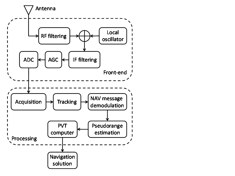Figure 1. Architecture of the considered software receiver

2.1. Acquisition Stage

In order to track and decode the information transmitted by the GNSS constellation, a generic receiver must at first detect the presence of the signal in space, performing the acquisition. The receiver must be able to search over a certain frequency range in order to cover all the expected Doppler frequency shifts on the received signal Once the acquisition algorithm detects the presence of the signal, two parameters must be estimated

• the delay τ of the received code with respect to the local code,

• the Doppler frequency shift f_d of the received signal (due to the relative velocity between the transmitting satellite and the user receiver).

The search space for acquisition operations must cover the full range of uncertainty in the code and Doppler offset. There are different methods to perform acquisition, based on the evaluation of the cross-correlation function of the received signal with a local signal, generated for each value of delay τ and Doppler shift f_d under evaluation (Cross-Ambiguity Function, CAF). Serial search (i.e., the cell-by-cell evaluation of the 2-dimensional CAF) is suitable for hardware receivers, due to its simplicity in implementation. Instead, in the perspective of a fully-software implementation, we focus on the parallel search in frequency domain, which exploits the Fast Fourier Transform (FFT), while serial search method is extremely slow for software-based implementation[21][22].

Indeed, methods based on FFT can be used to efficiently evaluate the correlation function. In the hypothesis to observe one code period (pre-detection integration T_int time equal to the code period T_c), the incoming sampled signal s_in[n] = s_in(nT_s) (where the sampling time T_s is chosen according to the GNSS signal specifications), is FFTtransformed, obtaining the sequence S_in[m] = S_in(m/T_s) = FFT{s_in[n]}.

A period of the current spreading code x is generated by the local code generator and it is stretched according to all the possible Doppler bins i, taking into account the minimum frequency resolution imposed by the time of observation T_int. The obtained signals are FFT-transformed, obtaining the sequences in the frequency domain.

The multiplications are then computed for each couple (x,i) in the frequency domain. After that, the inverse FFT (IFFT) is performed, so obtaining the circular correlation sequence. Its absolute value is computed and a possible peak in the delay domain is searched. This allows evaluating the relative delay of the spreading code for a certain Doppler shift step i.

This procedure has been performed to acquire both GPS and Galileo satellite signals. Of course, the code period T_c is different between the aforementioned GNSS signals. In case of E1-B this procedure has been performed to acquire both GPS and Galileo satellite signals. Of course, the code period T_c is different between the aforementioned GNSS signals. In case of E1-B Galileo signal we have a code length equal to 4ms as reported in[19] while the T_c in case of L1 C/A for GPS is 1ms[20].

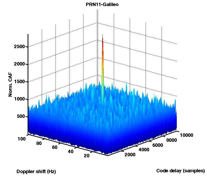Figure 2. Estimated CAF for Galileo PRN 11

The CAF obtained by using the latter acquisition technique to process the Galileo PRN 11 is shown in Figure 2.It is possible to identify a peak in the search space and it corresponds to the Maximum-Likelihood (ML) estimate of the Doppler shift and code delay. Such a method is well suited to be implemented in a real-time software receiver. For example, the N-Gene receiver is able to perform in parallel the initial acquisition of all the four satellite channels necessary for the first PVT fix.

2.2. Tracking Stage and Pseudorange Computation

Once the acquisition phase has brought the received and the locally generated code within less than a half chip period residual offset, a fine synchronization, named tracking, takes over and keeps the two codes aligned, by means of closed loop operations. Generally, the tracking system in GNSS receivers consists of a Delay Lock Loop (DLL) for code tracking and a Phase Lock Loop (PLL) for carrier phase tracking.

A detailed analysis of how a PLL and DLL work is out of scope of this paper and an exhaustive description can be found in[21]. The main aim of this Section is to stress the fundamental role played by the tracking stage in the correct and precise recovery of the code delay τ, which is necessary to measure the pseudoranges, and consequently the PVT solution, and to decode the navigation message. Focusing on the estimation of the pseudoranges, they are usually computed using two different methods.

1) The first technique (named common transmission time) is based on the satellites transmission time. In fact, all satellites broadcast data synchronously but, due to different propagation delays, at a given time the user does not receive the same data from every satellite.

Once each preamble is identified for all available channels, a comparison on their time of arrival is performed. In this case, in order to determine the set of pseudoranges for the first time, the channel with the earliest arriving subframe is assumed as a reference and a minimum travel time is assigned to the reference channel (e.g., its value, for GPS, is in a range between 65 and 85 ms). This concept is sketched in Figure 3.

All other pseudoranges are then derived respect to the reference channel through proper time counters, that are continuously updated by the tracking structures of each channel. If we suppose that the start of the subframe is identified for all the tracked satellites, then the receiver measures the time difference between the starting points of the subframe and the reference one. This time difference δ_i can therefore been written as , where represents the time of reception of the subframe for the i-th satellite while is the time relative to the reference satellite.

The time difference δ_i for each i-th satellite can be computed by means of specific time counters. Although there are many time-keeping conventions, which depend on the specific receiver implementation, the system of counters has to accumulate the number of words (i.e.: in case of the GPS C/A code, 1 word = 0.6 s), data bits (i.e.: 1 data bit = 20 ms), code periods (i.e.: 1 GPS C/A code period = 1 ms), and samples (i.e.: 1 sample = 1/sampling frequency ). In the case of Galileo, the procedure is similar to the GPS case. The receiver has to store the following parameters, in order to compute a valid pseudorange: number of pages (i.e.: 1 page = 2 s), data bits (i.e.: 1 data bit = 4 ms), code periods (i.e.: E1-B code period = 4 ms) and samples (i.e: 1 sample = 1/sampling frequency where is the same as the GPS’s one, as the receiver uses a unique front end to collect and digitalize the incoming GNSS signals). It is important to stress that receivers are able to measure the time offset with a resolution on the order of a fraction of chip (i.e.: a fraction of microseconds).

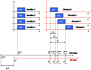Figure 3. Pseudorange computation based on transmission time

With these time differences, the pseudoranges can be written as , where is the bias between the clock of the user and the ones on board of the satellites, c is the speed of light, is the pseudorange relative to the reference channel and is the delay of the i-th satellite channel with respect to the reference satellite.

This kind of approach has some disadvantages to be implemented in a real-time fully software receiver:

a) Since the beginning of a given subframe transmitted by different satellites is received at different times, the receiver has to count for each tracked satellite the time elapsed from the reception of the subframe in the reference channel (i.e. the satellite with the shortest distance to the user’s receiver) to the beginning of same subframe for at least other three satellites. As a consequence, this kind of approach is not particularly suitable in a real-time implementation, since it requires to wait until all the channels have received the same data bit (e.g. the beginning of the same subframe) to compute the pseudoranges.

b) In case of a joint GPS/Galileo scenario, this technique is unsuitable in real-time implementations, since the receiver would have to work with two independent satellite systems, characterized by different data structures and two separate reference channels (one for GPS and one for Galileo). This approach will force the receiver to keep a large amount of information into its buffer, with a significant waste of resources as well as a non-negligible delay in the PVT computation. For this reason, it is useful to consider a different method, that takes into account the status of every channel at a given, unique time, fixed by the receiver.

2) The second approach (common reception time) performs the pseudoranges estimation by setting a common reception time over all the channels. In this case, which is sketched in Figure 4, the time elapsed from the reference bit (TLM in the Figure) to the bits currently considered in each channel (X, Y, Z, W in the Figure) is different for each channel, since the transmission time corresponding to the data message currently processed by the receiver is different for all the satellites.

The different time offsets are computed measuring the time passed from the reception of the last subframe and the receiving time instant set by the receiver as shown in Figure 4.

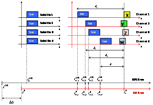Figure 4. Pseudorange computation based on transmission time

Also in this case, the channel with the lowest time counter is selected as the reference and its propagation delay is generally chosen in a range between 65 and 85 ms. All other channels will have a longer propagation delay, proportional to their distances. In this case, the time difference δ_i can be computed as , where is the time when the receiver computes the pseudoranges and it is common to all the tracked signals.

This method allows to obtain pseudoranges at any time, without waiting for a particular bit front on each channel, and it is often employed in commercial GPS receivers and is the technique that has been implemented in our joint GPS/Galileo receiver.

The effect on the final PVT accuracy of implementing these two approaches will be analyzed in Section III.

2.3. PVT Computation

The computation of the PVT can be demanded to many different algorithms. Nonetheless, this stage must be always provided with the following data, at least:

• Pseudorange measurements

• Doppler measurements

• Satellites related data (positions, errors, etc.)

The simplest method to implement the PVT stage of a GNSS receiver is to consider the Least Squares (LS) solution [21]. The rationale is to iteratively update the position solution at a given time, starting from a generic linearization point (usually the centre of the earth) and iteratively updating it to converge to the least squares estimate given by the current set of measurements. The linear equation stating the relation between the pseudorange prediction error vector, and the estimated position error, is the following:

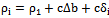
where is the difference between the measured and estimated pseudoranges, is the correction to be applied to the linearization point and the matrix is the Direction Cosine Matrix (DCM), whose rows are made up by the unitary vectors pointing from the linearization point toward each one of the satellites in view; the subscript pdr stands for ‘pseudorange’.

It must be noted that the pseudorange prediction error and the DCM are conceptually made of two parts. The upper part stores the values related to the GPS measurements, while the lower part stores the measurements related to Galileo. Moreover, the vector is made up by five elements:

where the first three components are the corrections in meters to be applied to the ECEF components of the linearization point, the last two are the clock bias corrections in meters to be applied to the GPS and Galileo clock bias linearization point, since the receiver must take into account a clock bias with respect to the GPS (upper part) and a clock bias with respect to Galileo (lower part), and T points out the transpose of the vector.

A similar result is obtained for the prediction of the velocity, when Doppler measurements are exploited [21]. In this case, the clock drift is the same for both the GPS and Galileo, so that the measurement matrix shows four columns:

and the corrections vector to the estimated velocity has four components:

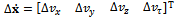where the first three components are the ECEF corrections in meters per second and the last component is the local clock drift correction in meters per second; the subscript dop stands for ‘Doppler’. The linear relationship between the pseudorange-rate error vector, and the estimated velocity error is then

Whenever a PVT solution has to be delivered, the LS iterations run to resolve the two linear systems written above.

Despite this method is simple, it has two main drawbacks. The first one is due to the complexity, since for each point the algorithm must usually iterate until the corrections are below a threshold and each time the pseudo-inverse matrix of (and ) must be computed. This issue might be avoided introducing a model to make the linearization point evolve, as in a Kalman filter.

The second drawback of the LS approach is due to the fact that the estimate is computed only on the basis of the current measurements, without any regards to the past trajectory and without weighting the available measurements. Despite the atter issue is solved using the Weighted LS (WLS), it is not possible to cope with the past trajectory using a LS-based method, ince it has no memory and at each time a solution is computed independently from the past.

For this reason, it is useful to adopt other methods that rely on the representation of state-space models [23-26]. Among these, the algorithm that historically has shown the best compromise between performance and complexity in GNSS receivers is the Extended Kalman Filter (EKF) [26], which is characterized by the following state-space equations:

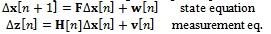where is the incremental state, is the state transition matrix, is the measurement prediction error, is the measurement matrix, is the process noise and is the measurement noise. The notation is in part similar to the one adopted in the LS discussion. This is a voluntary choice, since the two algorithms are based upon similar concepts. The incremental states represent the increments (corrections) to be applied to an a priori estimate of the state, which acts as a linearization point. The state model adopted here is characterized by nine incremental states, the first five related to position and the last four related to velocity:

to which the following state-transition matrix is associated:

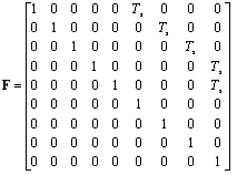Each time a new set of pseudorange and Doppler measurements is available, the Kalman filter is iterated once. The first step (prediction) allows to get the a priori estimate by using the last obtained estimate of the PVT in the state equation. This value is used to compute the prediction of the measurements and, together with the measurements, to compute the correction to be applied to the a priori estimate, as follows (update):

where is the Kalman gain. Finally, the a posteriori estimate is obtained correcting the a priori estimate:

The main advantage of the EKF with respect to the LS is the introduction of a method to balance the contribution of the trajectory given by the model and the one obtained by the measurement. In this way, it is possible to obtain a smoother trajectory than the one obtained using the LS and to avoid the model trajectory to diverge. A complete definition of this model can be found in [26] and [27]. These results will be analyzed in the following section.

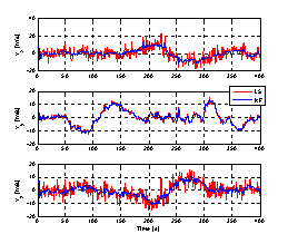
3. Comparative Results

In this Section we investigate the effects of the two different approaches to compute the pseudoranges discussed in Section II.B; then, we show some results we obtained by using both a LS and an EKF approach to resolve the PVT problem.

Concerning the calculation of the pseudoranges, an example of their estimation results by using the two methods of Section II.B is depicted in Figure 5, taking as an example the GPS satellite with PRN 30.

Figure 5. Comparison between pseudoranges computed by using common reception time and common transmission time

The blue ‘x’s represent the pseudorange computed by considering that all the satellite broadcast the same navigation data at the same Time of Week (TOW) (common transmission time). On the contrary, the red ‘+’s show the pseudorange as calculated by fixing a unique time of reception, that is set internally by the receiver (common reception time); as a consequence, the time of transmission of the navigation data is different for each satellite. Therefore, if we suppose to start the PVT computation at the beginning of a subframe and to update it every second, the pseudorange computed using the first method is measured when the time of transmission is equal to TOW. In the second case the pseudorange is computed at a transmission time that is not the same as TOW, but changes according to the reception time that has been fixed in the receiver. As discussed before, this latter approach allows to simplify the state-machine governing the operations of the receivers, as well as to reduce the memory occupied for the satellite channels in tracking.

In order to clarify this concept, in the two columns of Table I we show the TOW of the bit sampled in the reference channel, considering both the common transmission time and the common reception time methods.

Table 1. Transmission time of the considered bit front TIME OF TRANSMISSION[s] Common transmission time Common reception time 311736 311736.277662467 311737 311737.277664239 311738 311738.27766595 311739 311739.277667661 311740 311740.277669371 311741 311741.277671082 311742 311742.277672854 311743 311743.277674503 311744 311744.277676275 311745 311745.277677986

Even if these two methods are conceptually different, no significant differences can be noticed in the pseudoranges estimates, which are substantially similar, but shifted in time due to the different computation instant.

The solutions obtained using the two different methods appear similar and the variance in the accuracy of the position along the three axes X,Y,Z has the same magnitude in both cases. This fact proves once again that the benefit of using a unique time of reception is especially in speeding up the PVT computation and it is recommended for real time implementations since, while it does not change the receiver accuracy related to the estimate of the user position, it does not require to put any channel in a stand-by state (as told in Section II.B).

Once we stated that the two methods are equivalent, we can evaluate the differences between the results provided by the LS and the EKF algorithms. In the following experiments, we consider both the GPS and the Galileo signals present in the received Signal-In-Space. In Figure 6 we show the 2D estimated trajectory, obtained from a dataset that simulates a car in motion. The track has been simulated starting from the path obtained using a Novatel receiver tightly coupled with an Inertial Navigation System.

A difference between the solution provided by the LS filter and the smoother one estimated by the EKF can be noticed. As stated before, this improvement is obtained thanks to the adoption of the state-space model and of a system to weight the contribution of the model and of the measurements through the Kalman gain.

In order to better evaluate the differences between the two solutions, we analyse the zoomed area shown in Figure 6. We consider here a portion of straight road, a turning and the same straight road in the opposite direction. It is clear that the LS provides a trajectory which is noisy and is characterized by the presence of some outliers during the turning, making it difficult to clearly identify the path. On the contrary, the Kalman filter provides a smoother trajectory, where the street and the roundabout are clearly visible.

A similar result can be obtained whereas velocity is analysed. The estimated velocities along the three axes are shown in Figure 7.

In this case, the trend of the LS estimates is much noisier than the one obtained running the EKF. However, it can be observed that the estimate provided by the EKF happens to be a smoothed (i.e. filtered) version of the LS estimate.

4. Conclusions

This paper has discussed a receiver architecture that allows to simultaneously process the Galileo and the GPS signals in a software receiver. Despite this topic is known in literature, we focused our attention on some practical implementation details that are often disregarded when the theory is discussed.

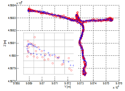Figure 6. Estimated trajectory, using both a LS (red circles) and an EKF (blue crosses) based receiver, and zoom of the north-western area.

Figure 7. Estimated trajectory, using both a LS and an EKF based receiver, and zoom of the north-western area.

The main effort of this work is towards the implementation of a joint GPS and Galileo receiver, in which particular attention has to be given to pseudorange generation and PVT computation.

At first, we dealt with pseudorange generation, considering two different methods, namely the common transmission time and the common reception time. In the results and in the description, we highlighted why these methods are equivalent from an accuracy point of view, what are their differences and why the common reception time method is more suitable for the integration of the two different satellites systems.

Furthermore, we considered both the LS filter and the EKF, which can be implemented to jointly process GPS and Galileo signals, describing the algorithms and the matrices that must be implemented.

Finally, we provided some comparative results related to the differences between the LS and EKF algorithm, to show why the EKF is nowadays the de facto standard when implementing GNSS receivers. Our results show that EKF perform better than a LS-based receiver in the case of both position and velocity estimation.