1. Introduction

A problem is suitable for binary classification when there are only two classes that the data needs to be divided into, and data samples are assigned to one of two classes based on a set of features or attributes. Machine learning models like Decision Trees, Bayesian Networks, k Nearest Neighbor, Random Forest, and others, have been used to build binary models based on assigning data instances to pre-assigned classes and then using this model to classify new instances. That is, given a set of data points and their corresponding labels, the machine learning model learns how they are classified so that when a new data point comes in, it is placed in the correct class (Shah, 2020). There are many real-world applications of binary classification, for example, classifying cancer patients as malignant or benign based on a set of features (Bagui, et al., 2003), classifying email as phishing or non-phishing based on email characteristics (Bagui, et al., 2019; Ma, et al., 2009), classifying network traffic as attack or normal based on a set of network features (Aksu, et al., 2018; Bagui, et al., 2021; Bagui and Woods, 2021, Syarif and Gata, 2017), etc. In this last scenario, the binary classification might be treated as a one class versus all classes scenario, with the one class being the normal network data and the other class (all) being all the different types of attacks grouped together as the other class.

In conventional binary classification algorithms, all features are treated as having equal weight and classification models are built without taking into consideration the fact that different attributes can have different levels of influence on a class. Weighted attribute classification is where different degrees of importance are assigned to different features in order to obtain a better classification model. Many variants of weighted attribute classification have been applied to conventional machine learning models to improve the correct classification rate (Singer, et al. 2020; Shahhosseini and Hu, 2021; Xiang et al. 2015; Ma, et al., 2020; Gajowniczek, et al., 2020; Biswas, et al., 2018).

To address the issue of weighted attribute classification, in this paper, we propose a feature weighting method based on mutual information. This attribute weighting measure is implemented on four classical machine learning classifiers, Naïve Bayes, k-Nearest Neighbor (k-NN), Decision Tree, and Random Forest. We evaluate our weighted classification models by comparing the performance of the weighted models to the performance of the traditional models (that is, the models without the weights).

The rest of this paper is organized as follows. Section 2 introduces some related works. Section 3 describes the methodology of several traditional binary classifiers in machine learning. Section 4 shows the weighting model we applied and our weighted classification approaches. Section 5 presents our experimental parameters, including computational parameters. In the computational parameters section, the libraries and functions applied are presented. Section 6 presents the results and discussion and finally the conclusion is presented in section 7.

2. Related Works

Several works have applied different forms of weighted attribute classification to machine learning models to improve the correct classification rate. Below we present works done on the Naïve Bayes classifier, Decision Tree, k-NN and Random Forest.

Works on the Naïve Bayes classifier: Wu et al. (2014) proposed a dual weighting method, attribute weighting and instance weighting, to improve the accuracy of the Naïve Bayes classifier. Zhang and Wang (2010) proposed a new weighted Naive Bayes method based on attribute frequency. Wu et al. (2015) proposed a method using immunity theory in Artificial Immune Systems to search optimal attribute weight values. These self-adjusted weight values alleviated the conditional independence assumption and helped calculate the conditional probability more accurately. Taheri et al. (2014) proposed using optimal weights determined by a local optimization method. Zaidi et al. (2013) proposed a weighted Naive Bayes algorithm that selected weights to minimize either the negative conditional log-likelihood or the mean squared error objective functions. Wu and Cai (2011) used differential evolution algorithms to determine the weights of attributes. Correlation coefficients were used by Yao and Li (2012) as the weighting measure in the Naïve Bayes algorithm. Xiang et al. (2015) handled the Naïve Bayes conditional independence assumption issue by using an attribute weighting method that employs the mutual information metric.

Works on the Decision Tree: In Polo et al. (n.d.), a weighted classification based on the decision tree algorithm was proposed to obtain simple yet accurate models. Farid and Rahman (2013) assigned weights to training instances in a decision tree based on posterior probability. Singer, et al. (2020) proposes a decision-tree model that applies a weighted information gain ratio for selecting and classifying attributes in a tree. This work is based on a weighted entropy function that uses a deviation of different classes. Suruliandi, et al. (2020) created a decision tree using ranks and weights of attributes assigned to branches based on their contribution towards classification accuracy.

Works on k-NN: In 0, several weight-setting methods for lazy learning algorithms were reviewed and a framework for distinguishing these methods was introduced. In Wolpert (1990), a weighted feature method was introduced based on information-theoretic approach for the nearest neighbor algorithm. Hechenbichler and Schliep (2004) introduced a weighting scheme for the nearest neighbors according to their similarity to a new observation that has to be classified. In Gupta (2012), a modified weighted attribute dynamic k-Nearest Neighbor classification algorithm using k-Means clustering is proposed. Sheikhi, et al. (2020) developed an efficient KNN classifier, WAD-KNN, that first uses a stepwise feature selection method to eliminate irrelevant features and then uses the number of N nearest neighbors that have a similar category, using the sum of their distances as a weight to improve the accuracy of the KNN algorithm. In other words, the class of each K nearest neighbors is multiplied by an efficient weighting method that guarantees the nearest neighbors contribute more to the final weight than the distant ones. Biswas, et al. (2018) puts a weight on each of the k nearest neighbors based on their distances from the actual point using a fuzzy membership function. Ma, et al. (2020) proposed a feature weight self-adaptive algorithm for weighted KNN and received better classification results.

Works on Random Forest: Shahhosseini and Hu (2021) propose several algorithms that modify the weighting strategy of regular random forest. Their weighting frameworks include optimal weighted random forest based on accuracy, optimal weighted random forest based on area under the curve, performance-based weighted random forest and several stacking based weight random forest models. Gajowniczek, et al. (2020) state that many studies have shown that a weighted ensemble can provide superior prediction results than simply average the decision trees in a Random Forest model. They propose a new weighting algorithm applicable to each tree in the Random Forest. Xuan, et al. (2018) focused on a weighting voting mechanism for Random Forest. Jain, et al. (2019) proposed a dynamic weighting schedule between test samples and decision trees in Random Forest where the correlation is defined in terms of similarity between test cases the decision tree using exponential distribution.

3. Methodology

3.1. Naive Bayes Classifier

The simplicity of the Naive Bayes classifier makes it a popular machine learning classifier. It continues to be effective on a wide range of classification problems, but the strong assumption that all attributes are conditionally independent given the class is often violated in real-world problems. Violation of this independence assumption can increase the expected error. We argue that the mutual information-based attribute weighting method should alleviate the conditional independence assumption in the Naïve Bayes algorithm.

3.1.1. Bayesian Theorem

Bayesian theorem describes the probability of an event given the prior knowledge of conditions that might be related to the event. It has been widely used in statistical inference. Let and be the events we are interested in, and are the marginal probabilities of and respectively, and are the respective conditional probabilities. Bayesian theorem is denoted mathematically by the following equation:

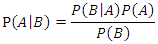
3.1.2. Naïve Bayes Classifier

The Naïve Bayes classifier is a typical machine learning model based on the Bayesian theorem with independence assumptions between the features. Suppose there are classes which are given an instance represented by a vector representing features, the classification is to assign this instance to the class which can maximize the probability of This can be derived from the Bayesian theorem as follows.

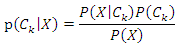As the denominator does not depend on the class and the values of features are given so that the denominator is constant. Thus,

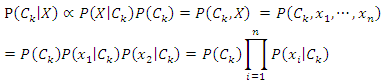The corresponding classifier is determined by the function that assigns a class label for some as follows:

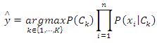
3.2. k-Nearest Neighbor Classifier

Though k-NN is generally a strong classifier, sometimes it does not perform as well as other classifiers. One reason for this is that each attribute has the same effect on the classification process and this causes less relevant characteristics to misclassify the class assignment.

k-NN is a lazy learning algorithm which stores the entire training set and does all the computations until it is time for classification. The classifier inputs a query instance and outputs a prediction for its class (0. Suppose we have a training set where is the instance denoted by a vector representing features and 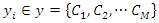is the class for each instance. Given a query instance , the classifier first finds a set of k-nearest neighbors, denoted as among the set of training set determined by the distance function . That is, k-NN calculates the distance of to each using:

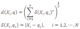Then, assign a class label to the query instance based on the decision rule. For example, if the decision rule is majority voting, the class label is determined by:

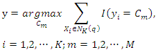where is an indicator function which yields 1 if the argument is true.

3.3. Decision Tree Classifier

Decision Trees are a powerful and popular machine learning classifier that use a tree-like model to make decisions. The goal of the decision tree algorithm is to create a model that predicts the value of a target variable based on several input variables. Once the decision tree construction is complete, it can be used to classify seen or unseen training instances.

3.3.1. Information Entropy

Suppose is a discrete random variable with finite possible values and probability mass function:

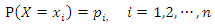The information entropy of can be denoted as:

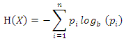where is the base of the logarithm used.

Similarly, the conditional entropy of two variables and taking values and respectively is obtained by:

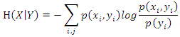where is the probability that and

3.3.2. Information Gain

The expected information gain is the change in information entropy from a priori state to a state that takes some information. Let be a set of training instances and be one of the features in the training set, then the information gain of given is denoted as:

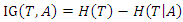Where is the conditional entropy of given the value of feature .

3.3.3. Iterative Dichotomiser 3 (ID3) Algorithm

ID3 is a commonly used decision tree algorithm. The ID3 algorithm begins with the original feature set as the root node. It iterates through each feature in the feature set and calculates the information gain of that feature, and then selects the feature which has the largest information gain as the root node. The selected feature is then used to split the data into several subsets based on the different values of the feature. The algorithm then takes each subset as a new dataset and continues to do this recursively with all features. The calculation of the information gain is as follows.

Suppose we have a training set with class labels and a feature A with the values of Let be the sample size of be the size of the samples that belong to class be the size of samples that have the feature value be the size of the samples that belong to class and have the feature value . Then the information entropy of the training set is:

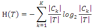The conditional entropy of given the value of feature is: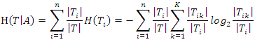

Thus, the information gain of given is: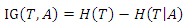

3.4. Random Forest

Random Forest is an ensemble learning model that deals with classification by constructing several decision trees at training time. Each individual tree in the random forest outputs a class prediction, and we take the class with the most votes as the prediction of the forest.

In a normal decision tree algorithm, we consider all the possible features and select the one that is the best in terms of splitting the data. For the decision tree in the random forest, however, each tree can only choose features from a random subset of features. This procedure ensures the variations among the trees and makes the decision of the random forest model more robust.

There are many ways to select the best feature to split the data. In this paper, we consider the split loss as our criteria to choose the best feature. That is, a feature’s performance objective in terms of splitting the data is to minimize expected loss. For every value of each feature in the random subset of features 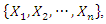first we use this value to split the data based on the class label and denote them as and representing the left-side data and the right-side data respectively. Then we compute the loss for the split data by:

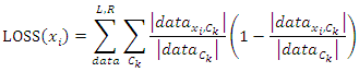Where is the number of instances in the data that belongs to the class label is the number of instances in the data that belongs to the class label and feature has the value

By comparing losses of different values, we choose the one that has the minimum loss as our best feature to build individual tree interactively.

4. Our Implementation

4.1. Mutual Information

4.1.1. Definition

Mutual information (MI) measures the mutual independence between two random variables. More specifically, it measures how much information we can learn about one random variable by observing the other random variable.

For two discrete random variables and the mutual information between them can be calculated as:

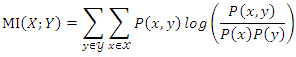Where is the joint probability mass function of and , and and are the marginal probability mass functions of and respectively.

For two continuous random variables the mutual information between them can be calculated as:

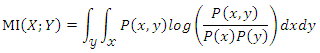Where is the joint probability density function of and , and and are the marginal probability density functions of and respectively.

4.1.2. Normalized Mutual Information

Suppose we have a dataset with a sample size of are two discrete features in this dataset, let and be the value of and respectively, and be the number of distinct values in feature and respectively, and be the number of instances that have the value of and respectively, be the number of instances that have the value of and at the same time. Then the normalized mutual information (NMI) between and is:

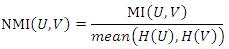Where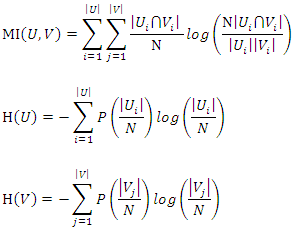

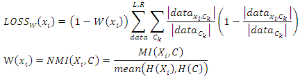
4.1.3. Converting Normalized Mutual Information to Feature Weights

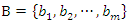
Feature weighting can be used to improve the classification accuracy in datasets where different features have different impacts on the class label. As mutual information is a measure of mutual independence between two variables, we consider the NMI between each feature and the class label as the weight of the feature. For example, suppose we have a dataset with instances, it has two discrete features and as well as a class label where 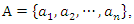and The weights of features and are defined as follows:

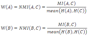Where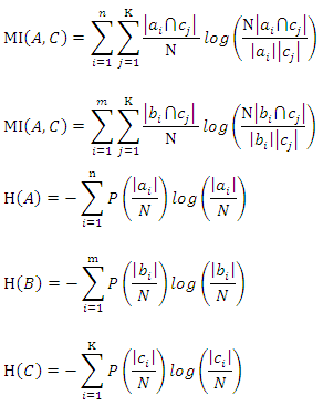

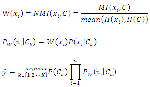
4.2. Weighted Naive Bayes Classifier

As mentioned above, in the Naïve Bayes classifier, all features contribute equally to the calculation of posterior probabilities. In real-world situations, however, this may not always be the case. In order to address this problem, we extend the conventional Naïve Bayes classifier to a weighted Naïve Bayes classifier by weighting the features when calculating the posterior probabilities. Our weighted Naïve Bayes classifier is presented in the following equations:

4.3. Weighted k-Nearest Neighbor

In the k-NN classifier, we integrate the weighting method into k-NN by defining a new weighted distance function. The weighted k-NN computes the distance between an instance and a query using:

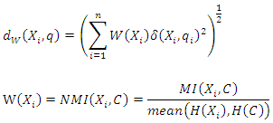We denote the new set of k-nearest neighbors found by the weighted distance function as Given a query instance , the class label of this query is determined by:

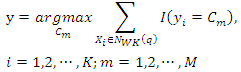where is an indicator function which yields 1 if the argument is true.

4.4. Weighted Decision Tree

As we mentioned earlier, the ID3 algorithm determines the best feature on which to split the data and builds the decision tree by comparing the information gain of the different features. However, the different features may have diverse impacts on classification. Taking this into consideration, a new way of calculating the conditional entropy by adding weights to the probabilities is proposed.

The weighted conditional entropy of dataset with class label given the value of feature is: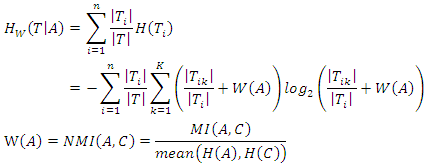

Thus, the weighted information gain of given is: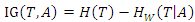

Our weighted ID3 algorithm chooses the best feature to build the decision tree by comparing the weighted information gain iteratively.

4.5. Weighted Random Forest

The loss function defined in Section 3.4 assumes that the loss of every feature value is related only to the variance of the split data. However, if the feature that we chose has more information about a class label than other features, it is reasonable that less loss should be assigned to this feature. Thus, in our weighted random forest classifier, we adjust the loss function by:

5. Experimental Parameters

This section explains the datasets used, the performance evaluation parameters as well as computational parameters for this experiment. Since binary classification is widely used in the medical scenario, we evaluate our weighted machine learning models with two medically related datasets from UCI (University of Wisconsin) Machine Learning Repository: (i) Wisconsin Breast Cancer (WBC) database (Mangasarian and Wolberg, 1990); and (ii) Blood transfusion service center dataset (Yeh et al. (2008)).

5.1. Description of the Datasets

The Wisconsin Breast Cancer (WBC) database was obtained from the University of Wisconsin Hospitals, Madison by Dr. William H. Wolberg (Mangasarian and Wolberg, 1990). This database contains 699 instances, among which 241 are malignant cases and 458 are benign cases. The original database has 16 instances which have some missing values. We removed these observations from the original database and conducted our experiments using the rest of the 683 instances. The reduced database has 239 malignant instances and 444 benign instances. The WBC database contains the following features: (i) Clump thickness; (ii) Uniformity of cell size; (iii) Uniformity of cell shape; (iv) Marginal adhesion; (v) Single epithelial cell size; (vi) Bare nuclei; (vii) Bland chromatin; (viii) Normal nucleoli; and (ix) Mitoses.

The Blood transfusion service center (BTSC) dataset was taken from the Blood Transfusion Service Center in Hsin-Chu City in Taiwan (Yeh et al. (2008). This database contains the information of 748 donors that were randomly selected from the donor database. This dataset includes four attributes and a variable representing the class label. The variables are: R (Recency – months since last donation), F (Frequency – total number of donation), M (Monetary – total blood donated in c.c.), T (Time – months since first donation), and a binary variable representing whether he/she donated blood in March 2007 (1 stand for donating blood; 0 stands for not donating blood).

5.2. Performance Evaluation

The performance evaluation of our weighted Naïve Bayes, weighted Decision Tree as well as weighted Random Forest are carried out based on the cross-validation, and the average accuracies were calculated for performance measurement. Several cross-validations with different folds, 3-fold to 11-fold, were applied in our experiments. For example, the 5-fold cross-validation divides the dataset into 5 subsets and one of the 5 subsets is used as the test set while the other 4 subsets are used as the training set each time. Thus, each fold as a test set has an accuracy value. We take the average value of these accuracies as the performance measurement of the corresponding approach.

For the weighted k-NN model, instead of using cross-validation, we conducted our experiments based on different k values, 1, 3, 5, 7, and 9. The accuracies of the different k values for k-NN and weighted k-NN were compared as well as the average accuracy.

5.3. Computational Details

Python was used to build the algorithms. In this section, we introduce the libraries, modules as well as functions applied in our algorithms for preprocessing as well as computing.

5.3.1. Data Preprocessing

The data preprocessing used for the two datasets was similar. The dataset was input as a data frame into our workspace, then split into features and true labels. The features were used to estimate the predicted labels, and the predicted labels were compared to the true labels to get the accuracies. The pandas library was used for this. The instances with missing values (16 instances) were removed from the WBC dataset, that is, from the data frame, before splitting the dataset. The dropna function in pandas was used to remove the instances with missing values.

5.3.2. Computing

The numpy library was used to do the calculations. The np.multiply.accumulate function was used to calculate the post probability in Naïve Bayes Classifier; the np.tile function was used to repeatedly calculate the distance between instances in the KNN method; the log function was used to calculate the Shannon entropy in Decision Tree algorithm. The sklearn library was also used. The normalized_mutual_info_score function in the metrics module from the sklean library was used to calculate the normalized mutual information between each feature and the true label for all the algorithms. The random module was used in the Decision Tree and Random Forest algorithm. In the Decision Tree, once the tree is built, the values of features in the tree are fixed, so it may be possible that an instance coming in cannot be predicted by the Decision Tree as the values of the features in this instance may not be the same as those in the tree. To solve this problem, the choice function was used to choose a random label for these types of instances. In the Random Forest algorithm, the randrange function was used to randomly choose a certain number of features from all the features to build the individual tree.

5.3.3. Output

To compare the performance of the original algorithms with our weighted algorithms, the output was set as the accuracy. This was done using the “if” loop and the logical operation to compare the predicted label with the true label for each instance.

6. Results and Discussion

The performances of our weighted machine learning models, Naïve Bayes, k-NN, Decision Tree and Random Forest, are compared to their respective conventional models.

6.1. The WBC Database

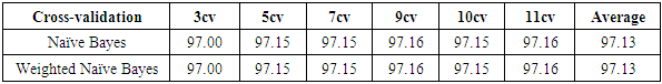
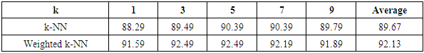
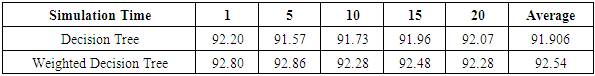
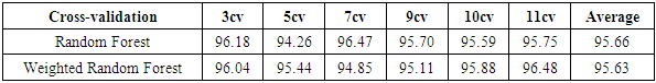
The results of the comparisons of the four conventional models to our respective weighted models using the WBD database (Mangasarian and Wolberg, 1990) are presented in Tables 1, 2, 3 and 4.

In Table 1, for the Naïve Bayes classifier, the classification accuracy for each cross-validation and the average accuracy for the weighted approach are presented. Our weighted Naïve Bayes model performs as well as the conventional Naïve Bayes model for all the different cross-validations, hence the average performance is also similar, at 97.13%.

Table 2 shows the correct classification rate for each k-NN with different k values and the average accuracy for the two approaches, conventional k-NN and weighted k-NN. The highest accuracy of the conventional k-NN model was 90.39%, while the highest accuracy generated by our weighted k-NN model was 92.49%. Moreover, the average classification accuracy was 89.67% for the conventional k-NN model and 92.13% for our weighted k-NN model. The weighted k-NN model performed better than the conventional k-NN model.

For the Decision Tree model, we applied 5-fold cross-validation with different simulation times and calculated the average classification accuracy for each simulation time. Table 3 reveals that our weighted Decision Tree approach outperforms the conventional model for each simulation time and for the overall average classification accuracy.

From Table 4, we can see that the average accuracy of the conventional Random Forest was 95.66%, which is slightly higher than the average accuracy produced by our weighted Random Forest 95.63%. However, our weighted Random Forest approach performs better than the conventional model as the folds of the cross-validations increase. The highest accuracy of 96.48% was obtained by our weighted method at the 11-fold cross-validation.

Table 1. Classification accuracies (%) for Naïve Bayes

Table 2. Classification accuracies (%) for k-NN

Table 3. Classification accuracies (%) for Decision Tree

Table 4. Classification accuracies (%) for Random Forest

6.2. The BTSC Database

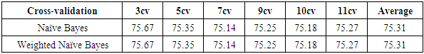
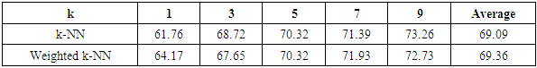
The results of the comparisons of the four conventional models to our respective weighted models using the Blood Transfusion database (Yeh et al., 2008) are presented in Tables 5, 6, 7 and 8.

As with the WBC database, our weighted Naïve Bayes model performs as well as the conventional Naïve Bayes model with an average accuracy of 75.31%, as shown in Table 5. Also, there is no difference in the classification accuracy of the different fold cross-validations for these two approaches.

From Table 6, we can see that our weighted k-NN model slightly outperforms the conventional k-NN in terms of average accuracy. The correct classification rate of the weighted k-NN increases by 2.41% when .

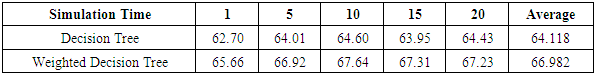
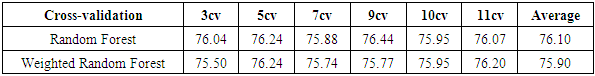
Table 7 shows that our weighted Decision Tree performs better than the conventional model. For the 5-fold cross-validation, the correct classification rate improves by 2.96% when our weighting approach is used.

For Random Forest, according to Table 8, the average accuracy for different fold cross-validations is 76.10%, which is slightly higher than the average accuracy of our weighted Random Forest. This might be caused by the random selection of features during the training process of Random Forest. If the algorithm happened to choose features that do not have a strong correlation with the class label, our weighting method might not work as well as the conventional approach.

Table 5. Classification accuracies (%) for Naïve Bayes

Table 6. Classification accuracies (%) for k-NN

Table 7. Classification accuracies (%) for Decision Tree

Table 8. Classification accuracies (%) for Random Forest

7. Conclusions

In this paper we evaluated a feature weighting method based on mutual information and conducted our experiments on four classical machine learning methods. Our empirical evaluation compared the performance of our weighted approaches to the original models.

Our findings suggest that our weighted approach performs as well as or better than the conventional methods, for the Naïve Bayes, k-NN and Decision Tree classifiers. For Random Forest however, the weighted approach did not perform better than the conventional approach. As for the k-NN model, the empirical study shows that the weighted k-NN performs better than the original k-NN model for both databases. Since the k-NN model is a nonparametric classifier, it can be applied to any data set (Bagui et al., 2003). The results of the weighted Decision Tree show an increase in accuracy compared to the conventional Decision Tree model, which indicates that our weighting method improves the traditional classifier. As an ensemble learning method for classification, Random Forest is supposed to correct the issues of overfitting to the training set which is a drawback that Decision Tree has. However, our empirical study shows that the weighted Random Forest slightly degrades the performance of the conventional Random Forest model. More investigation needs to be done to understand this result.