Ali Obied
Faculty of Computer Science & Information Technology, University of Sumer, Iraq
Correspondence to: Ali Obied, Faculty of Computer Science & Information Technology, University of Sumer, Iraq.
| Email: |  |
Copyright © 2017 Scientific & Academic Publishing. All Rights Reserved.
This work is licensed under the Creative Commons Attribution International License (CC BY).
http://creativecommons.org/licenses/by/4.0/

Abstract
The design of systems, or agents, situated in dynamic environments is of considerable practical and theoretical importance. This paper describes experiments examining the efficacy of dynamic sensing policy when the time cost of processing sensor information is significant. Extending the TILEWORLD experiments performed earlier by Obied, et al. in [1] this article produce interesting development of EBDI-POMDP agent by integrating among knowledge base models, decision theory and Self-Organizing system. This article clear distinguishes between sensing policy and sensing cost, since; it described experiments examining the efficacy of dynamic sensing policy when the time cost of processing sensor information is significant. It is demonstrates that several expected features of sensing cost and planning cost do arise in empirical tests. In particular, it is trying to answer the question is how would scalability of agent improve? The observations that for a given sensing cost and degree of world dynamism, an optimal sensing rate exists and, it is shows how this optimal rate is affected by changes in these parameters.
Keywords:
Situated agent, Extensible beliefs desires and intentions, Partial observable markov decision process
Cite this paper: Ali Obied, Deliberative Regulation with Self-Organising Sensing, Advances in Computing, Vol. 7 No. 3, 2017, pp. 80-94. doi: 10.5923/j.ac.20170703.03.
1. Introduction
Situated agents are artificial systems capable of intelligent, effective behaviour in dynamic and unpredictable environments [2]. Their design raises important theoretical and practical questions about the optimal control of reasoning with limited computational resources. Previously, Obied and others presented a paper describing theoretical and empirical studies of self regulation for situated agents in [1]. The experimental system was a modification of the TILEWORLD [3] coupled with the EBDI real-time reasoning system [4]. In this domain an agent is repeatedly confronted with the choice of whether or not to replan; that is, to recompute its optimal course of action. The results reported showed that when the cost of replanning is significant, the optimal strategy is to replan reactively, when the environment has changed in an important way that renders invalid previous decisions and commitments. To successfully implement a reactive replanning strategy, an agent must be able to determine when such changes have occurred. In the TILEWORLD, certain observable events are reliable indicators of significant change. The experiments reported made the simplifying assumption that the agent had perfect knowledge of the current state of the world, and could detect these events at no cost. This is obviously unrealistic as a model of an agent with real sensors. Although sensors can run in parallel with reasoning systems, processing the output of the sensing can have costs in terms of reasoning time. In addition, the certainty of sensing information can increase when additional time is spent on further processing. When the cost of sensing is significant, an agent cannot afford to incur this cost too frequently. Costly sensing is no different, in some ways, from costly replanning; the optimal strategy is to reactively sense just when there is some interesting feature in the environment to observe. Unfortunately, in most domains this strategy is not practical, as there are no reliable low-cost indicators that can be used to trigger sensing. Thus agent designers, and possibly agents themselves, must make decisions about how and when to schedule sensing. These decisions are critical to realistic planning/acting systems and autonomous agents such as the NASA Mars Rover [2]. Designing sensing policies has become a focus for recent work; for example, that of Chrisman and Simmons in [5] which argues for static sensing policies, where decisions about when to sense are made in advance by agent designers in order to reduce planning complexity, the work of Abramson in [6] which presents a decision theoretic analysis of how often to sense for errors that may occur during plan execution, and the work of Kinny and others in [2] which argues static sensing policy in specific level of dynamism, and their results indicate that static sensing policies can be successful, provided that the rate of change in the environment and the cost of sensor processing do not vary too greatly. But it can be dangerous to extrapolate the results of experiments of this nature to more complicated domains that involve complex sensing strategies and noisy and uncertain sensors such as those used by real robots, the effects observed do seem to support the hypothesis that static sensing policies can be effective, provided that the rate of change in the environment and the cost of sensor processing don't vary too greatly [2].Given the important interactions between sensing, planning and action, we have extended the methodology developed by Kinny and others in [1] to model agents that incur significant sensing costs. The aims of authors in this paper, was to measure experimentally various predicted effects that arise due to sensing cost, and to examine the sensitivity of dynamic sensing policies to variation in the rate of change in the world, the cost of sensing and the world size. Furthermore, they extended the experiments in [1] for planning cost in different circumstances; increasing the rate of world (complex environment), increasing the size of world and the cost of planning. In this paper, we may find the answer of the question is how would scalability of agent improve?• Sect. 2 describes the background and relevance domains, sect. 3 presents formal framework,• Sect. 4 describes empirical validation with some questions and their answers to support the method and the final section presents the conclusions and future work.
2. Background
2.1. Extensible Beliefs Desires and Intentions (EBDI) Model
The proposed EBDI provides a highly suitable architecture for the design of situated intentional software that continuously monitors and/or observes its environment and acts in accordance with its situated BDI, grounded in a normative settings [4]; Beliefs correspond to service information derived and/or accessed from a range of sources, including; domain, environment or the beliefs of other services.Desires represent the state of affairs in an ideal world, which often maximise the service's own goals. By comparing a system’s beliefs set (observed system states) against its desires, the system detects a mismatch and triggers a set of intentions [7].Situated intentions represent an action set for the system to undertake in a given situation to achieve its specified desires, and /or to address the mismatch between the system’s environment (beliefs) and system’s goals (desires).Normative intentions represent a set of actions to be undertaken to ensure a specified set of norms including obligations (deontics), and rule representations are observed before a given intention is enacted. Also, maintaining the integrity of emerging rules.Utility intentions represent a set of actions to optimise goal-oriented intentions [4]. This means that at any point an agent may find itself with a number of competing intentions. In the first instance this may be a conflict over whether to act or to deliberate. Further intentional conflicts will arise as the agent seeks to comply with its personal norm set (ontology), the global norm set (shared ontology) and its obligations to itself and other agents. Some of these competing intentions may even be contradictory. Methods for optimising an agent’s decision processes, so that the action with the highest reward for the system is completed, have been studied for some time [8]. However defining and implementing functions that provides a notion of action utility is very problematic. The complete specification can consist of a very large (even infinite) number of perception-action pairs, which can vary from one task to another [9]. Also the terms ‘agent’ and ‘environment’ are coupled, so that one cannot be defined without the other. In fact, the distinction between an agent and its environment is not always clear, and it is sometimes difficult to draw a line between them [10].
2.2. Partial Observable Markov Decision Processes
A partially observable Markov decision processes POMDP is a generalization of an MDP. It assumes that the effects of actions are nondeterministic, as in MDPs, but does not assume that feedback provides perfect information about the state of the world. Instead, it recognizes that feedback may be incomplete and environmental data is subject to uncertainty. Due to this, a POMDP is said to be partially observable [11]. To see why this extension is important, consider the interactions between an agent modelled by POMDP and its environment. On one hand, the world states can be changed by executing actions. This procedure can be viewed as the control effects of actions. On the other hand, a feedback is provided to the agent when the world states change. This procedure can be viewed as the information-gathering effects of actions since different actions can change the world to different states and in turn this allows the agent to receive varying feedback [11]. Therefore, POMDP provides a unified framework to handle these two sources of uncertainties: the control effects of actions and information-gathering effects of actions. Hence, POMDP provides a method of making tradeoffs between choosing actions to change the world states and actions to collect information for the agent. Thus, a method is presented that takes into account the risk associated with a given circumstance and allows the agent to gather and utilize data to maximize its expected reward or minimize unpredictability and maximize safety.
2.3. TILEWORLD
TILEWORLD was initially introduced in [3] as a system with a highly parameterized environment which could be used to investigate reasoning in agents. The TILEWORLD is inherently dynamic: starting in some randomly generated world state, based on parameters set by the experimenter, it changes over time in discrete steps, with the appearance and disappearance of holes. An agent can move up, down, left, or right, and can move tiles towards holes. The experimenter can set a number of TILEWORLD parameters, including: the frequency of appearance and disappearance of tiles, obstacles, and holes; the shape of distributions of scores associated with holes; and the choice between hard bounds (instantaneous) or soft bounds (slow decrease in value) for the disappearance of holes. In the TILEWORLD, holes appear randomly and exist for as long as their defined life-expectancy, unless they disappear because of the agent's actions. The interval between the appearance of successive holes is called the hole gestation time.The TILEWORLD agent is a 2-dimentional grid on which an agent scores points by moving to targets, known as holes. When the agent reaches a hole, the hole is filled, and disappears. The task is complicated by the presence of fixed obstacles. The TILEWORLD is four connected, that is the agent can move horizontally or vertically, but not diagonally. A lower bound on the shortest path length between two points is thus given by the Manhattan distance 
2.4. EBDI-POMDP Agent
EBDI-POMDP agent has argued in [1] which has provided a model-based regulation mechanism to support planning in unknown dynamic environments. It has applications to danger theory with deliberative and anticipatory support to respond to environmental triggers. In this way deliberation is a response to danger signals with intentions set and reviewed based on the benefits (utility) that may accrue from enacting these intentions. In other words, reaction of autonomic systems’ to a known stimulus has to be analyzed based on logics, deontics reasoning and overall effect (or utility). So actions may be selected for predictability and safety by a rigorous risk assessment being performed at each agent autonomously –defined, deliberation cycle. That is the agent selects its intentions based on the best available data to optimise the system’s operation. Additionally the agent is capable of reviewing its own operation in terms of optimising its observe-deliberate-act sequence. Theoretical and experimental work into an efficient and effective reconsideration of intentions in autonomous Extended Belief-Desire-Intention (EBDI) agents was presented. The framework integrates an abstract EBDI agent architecture with decision theoretic approaches; Partially Observable Markov Decision Processes (POMDP). Agents were used as proactive autonomous social entities that can adapt to environmental changes and solve problems, which they encounter during execution, with limited or no human intervention. The conclusion of this work that the knowledge base is not scalable in highly dynamic worlds; however, interesting future work which mentioned in [1] includes investigating ways to develop methods for the agent to improve its behaviour in complex domains. For this the POMDP-EBDI agent is a promising candidate to facilitate rigorous logical monitoring and tending of large complex systems.The POMDP framework is used a domain independent meta level reasoning component, which let the agent to control the process by EBDI model. Meta level EBDI-POMDP defined as 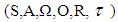 . Where the state s
 S in this model denotes an internal state of the agent, containing a belief part and intention part, actions and rewards, Ω denotes the observations, the observation function O, and the state transition function
  to designer for now.Since the POMDP used to model EBDI, the agent either performs an object level action (act) or the agent deliberates (del) [1].Thus A={act,del} denotes whether the agent acts or deliberates. Because the optimality criterion of policies depends on the reward structure of the POMDP, the rewards for action act and deliberation del in state sS define as follows:
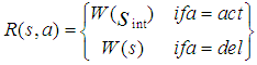 | (1) |
Where  refers to the state the agent intends to be in while currently being in state s.With respect to this last intuition, however, must mention that the real reward for deliberation is indirectly defined, by the very nature of POMDP, as the expected worth of future states in which the agent has correct intentions.As intentions resist reconsideration, the agent prefers action over deliberation and the implementation of the reward structure should thus favour action if the rewards are equivalent.
2.5. Self-Organising System
The essence of self-organization is that system structure often appears without explicit pressure or involvement from outside the system. In other words, the constraints on form (i.e. organization) of interest to us are internal to the system, resulting from the interactions among the components and usually independent of the physical nature of those components. The organization can evolve in either time or space, maintain a stable form or show transient phenomena. General resource flows within self-organized systems are expected (dissipation), although not critical to the concept itself. The field of self-organization seeks general rules about the growth and evolution of systemic structure, the forms it might take, and finally methods that predict the future organization that will result from changes made to the underlying components. The results are expected to be applicable to all other systems exhibiting similar network characteristics. The main current scientific theory related to self-organization is Complexity Theory, which states: "Critically interacting components self-organize to form potentially evolving structures exhibiting a hierarchy of emergent system properties" [12].The elements of this definition relate to the following: • Critically Interacting - System is information rich, neither static nor chaotic • Components - Modularity and autonomy of part behaviour implied • Self-Organize - Attractor structure is generated by local contextual interactions • Potentially Evolving - Environmental variation selects and mutates attractors • Hierarchy - Multiple levels of structure and responses appear (hyperstructure) • Emergent System Properties - New features are evident which require a new vocabulary.For more details see [12].
3. Method
3.1. Self-Organizing via EBDI-POMDP Agent
Interesting developments of EBDI-POMDP agent when dynamism increasing is integrate it with Self-Organizing system, to diagnose complex environment's changes to decrease the uncertainty. In other words, we argue how can we develop EBDI-POMDP agent to do so in complex environment (variable change), when the environment indeterminist (when the agent is equipped with incomplete world description in terms of dynamism)?Also, we need to know; if we increase the level of dynamism how will be the agent’s behavior? To answer these questions the authors integrate self organizing system with EBDI-POMDP agent as two layers working together for this task. First layer represents many simple agents, to read and send the information as perception to beliefs set of EBDI-POMDP agent which represents the second layer.
3.2. General Framework
In this section we formalize general development of our framework to diagnose risk and or benefit of above idea as observer architecture, and in the next section we formalize the idea for TILEWORLD simulation. Suppose we have system that finite set of properties X and suppose we know the initial values of them. Furthermore, if non-self enter the environment and there is a change in such property the state of property will change (ON or OFF) according with (appear or disappear of hole in TILEWORLD).So, to do self regulation by Self-Organizing system to diagnose non-self entity that entered the environment as a risk or benefit we need to do two steps as follow:1- We need to determine signal zone, in other words determine specific system properties that already changed after non-self entered the environment (attention switching).2- We need to know what that change represent is for whole system, such as a risk or benefit?To do above steps we will use two layers of agents.• Firs Layer This layer contains number of simple agents embedded in nodes as fixed reader agents, in other words, each node includes one simple agent to read and send the value of property at any time. Suppose we have finite set of properties X which represents all system properties, since  | (2) |
Let  , represents the set of properties may be changed or not after non-self entered the environment. N represents number of all cells (nodes).Now, we can use fixed simple agents to determine
  . The simple agent which embedded in each node will read the value of property and it save triple
  and send
  to EBDI-POMDP agent’s beliefs, since,
 Represents the value of property
  before non-self entered the environment (initial value of
  ).
). Represents the value of property
  after non-self entered the environment.
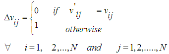 | (3) |
After we finish this step will have set of properties that concerning with the change in environment (attention switching), to send it as matrix information to EBDI-POMDP agent’s beliefs. • Second LayerThis layer uses the knowledge base model EBDI-POMDP agent and backward information as artificial immune system to determine the changes in specific properties, either represent a risk or benefit by the same diagnosing way which done in [1], but with decreasing the uncertainty which yields from combining Self-Organizing system to model.
3.3. Framework via TILEWORLD
This section presents formal model’s parameter in TILEWORLD. Let , represents the states set of cells (appearance or disappearance of hole) in TILEWORLD, since N represents number of cells in TILEWORLD.
 represent the set of cells except obstacle’s cells.
 | (4) |
 represents the state of cell when hole OFF.
 represents the state of cell when hole ON.In this moment it is possible to use number of simple agents embedding in TILEWORLD cells except cells which already have obstacle. Each cell includes simple agent k which defined as follow:
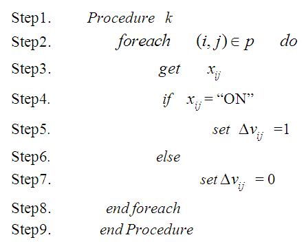 | Figure 1. Shows fixed simple agents in TILEWORLD to read value of each cell |
By steps from Step1-Step3 in Fig.1, we will get information from all cells in p, by steps from Step4-Step7 we will decide if the state of hole appearance or not.Now,  in Eq.3 can redefine as follow:
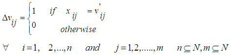 | (5) |
and  represents the state of hole in cell
  The effect of this process will be matrix for all agents
 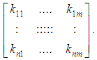 For instance
 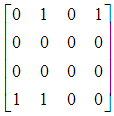 means, there are 4 holes appearance in our small grid in this example and the locations of these holes are; (1,2),(1,4),(4,1) and (4,2). So, EBDI-POMDP agent will chose closer hole of it location to fill it as we explained in sect. 2.3.
4. Empirical Investigations
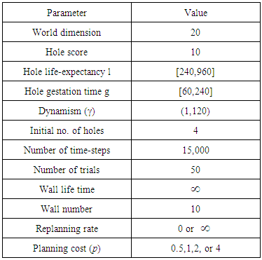
The TILEWORLD is easy to implement, but still offers enough complexity to investigate research questions. Additionally, for the development of theoretical ideas on such research questions, the TILEWORLD offers a very intuitive domain to concretely formulate otherwise very abstract concepts. The task of an agent in the TILEWORLD is to visit holes in order to gain as many points as possible. The agent decides which hole to visit based on hole distances - it always chooses to visit the nearest hole. The same simplifications used in the original TILEWORLD of Kinny and Georgeff [13] and Obied and others [1] are assumed here except some parameters such as increasing dynamism, adding sensing cost in some experiments.Following [13] and [1] the effectiveness ε of an agent is defined as the ratio of the actual score achieved by the agent to the score that could in principle have been achieved. This measurement is thus independent of the randomly distributed parameters in a trial. Also, the Dynamism γ (an integer in the range 1 to 120 denoted by γ) represents the ratio between the world clock rate and the agent clock rate. If γ =1 then the world executes one cycle for every cycle executed by the agent. Larger values of γ mean that the environment is executing more cycles for every agent cycle; if γ > 1 then the information the agent has about its environment may not necessarily be up to date In Table 1 an overview of the values of relevant parameters that were used in the experiments are given;  denotes a uniform distribution from
  to
to  and
and  denotes the range from
  to
to  . Note that each TILEWORLD was run for 15,000 time steps, and each run was repeated 50 times, in order to eliminate experimental error. Wall represents obstacles, hole life expectancy l represents hole age before it disappear and gestation time g represents elapsed time between two successive appearances of holes.
Table 1. Overview of the experiment parameters
 |
| |
|
4.1. EBDI-POMDP-SO
This section produces new version of EBDI-POMDP agent, so to distinguish between new agent and other agent which used in [1], let us call new agent in this section as EBDI-POMDP-SO agent. Solving Self-Regulation agent (EBDI-POMDP-SO) for TILEWORLD domain delivers an optimal domain dependent reconsideration strategy: the optimal EBDI-POMDP-SO policy lets the agent deliberate when a hole appears that is closer than the intended hole (but not on the path to the intended hole), and when the intended hole disappears. The experiment results shown in Fig.2, our results in this Figure is overall better than results as obtained in [1], as a result from combining Knowledge base and Self Organizing System.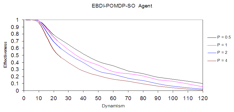 | Figure 2. Shows Self-Regulation (EBDI-POMDP-SO) Agent in TILEWORLD |
Self-Organizing System represents the first layer of EBDI-POMDP-SO agent as a parallel search algorithm to provide good awareness (sensing) about environment, and send this information to EBDI-POMDP which represents a second layer of EBDI-POMDP-SO agent. In addition, we can see in Fig.2 high dynamism of TILEWORLD about 120, which represents high complex environment rate with clear improvement of agent behaviour.However, the agent succeeds in filling those holes whose life-expectancy are sufficiently long, and even in highly dynamic world; there will some holes that meet these criteria. Also the agent may success fill only some small fraction of the holes.In Fig.3 it is clear to see the different between the two agents and EBDI-POMDP-SO outperforms other agent depending on planning time cost. The deferent between behaviors resulted from knowledge received from sensing operation which represents better than general knowledge which used in EBDI-POMDP agent without sensing operation. 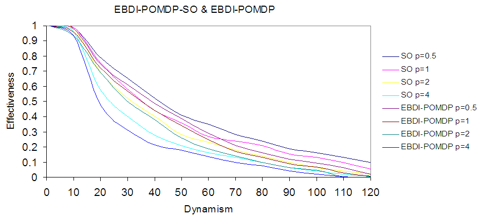 | Figure 3. Shows the comparison between EBDI-POMDP-SO agent and EBDI-POMDP agent which presented in [1] when p=0.5, 1, 2 & 4 |
4.2. Sensing Policy
Unlike the above experiment that assumed the sensing cost to be nil, this test will evaluate the EBDI-POMDP-SO agent's behaviour if this cost was not zero. To this end, a brief comparison between EBDI-POMDP and EBDI-POMDP-SO models is required. Whereby, if sensing cost is zero (or sensing is free) the EBDI-POMDP agent will request sensing information at every step. However, if sensing is not free this process will be expensive, hence, the agent will have to deliberate to determine how and when sensing information is queried. In other words, an optimal sensing policy for EBDI-POMDP agent will be required. Hence, we suggest adding the new agent as a filter to evaluate and analyse sensing information an event before they are sent to EBDI-POMDP agent (the upper layer). Thus, the observer (filter) represents middle layer between simple agents and EBDI-POMDP agent. Such a filtering process can be outlined as follows:Simple agents (or self-organising particles) scan the environment and broadcast the environment state according to a defined policy. For instance, sending the state of a given hole at a regular clock cycle. Filter evaluates the environment state information and send them to EBDI-POMDP agent in accordance with a defined filtering policy. For instance, if the environment state changed.Observer receives feedback from EBDI-POMDP agent concerning which hole was visited.Fig. 4 shows the observer algorithm, in which the observer in Step1 beliefs of EBDI-POMDP agent, Step2 to Step4 get information from simple agents that scan the environment and sending the information to observer at any moment of time. In Step5 to Step9 the observer evaluates the information about the environment by Boolean algebra function and send information as beliefs set to EBDI-POMDP agent if the information is important (i.e., in TILEWORLD if new hole appears closer than intended hole or if intended hole disappears), and end the process if not.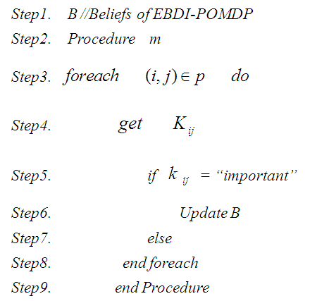 | Figure 4. Shows observer algorithm |
The solution of the sensing policy and cost will follow the same method in section 3.3 for computing the planning cost and policy. Thus A = {send, end} denotes whether the agent sends information to Beliefs set or end sensing processes. Because the optimality criterion of policies depends on the reward structure of the POMDP, the rewards for action send and end the sensing process end in state sS define as follows: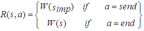 | (6) |
Where  refers to the state of the information is important (some new hole appear or intended hole disappeared) to be in while currently being in state s. It is important to mention again EBDI-POMDP agent receives perception as beliefs depending on a sensing policy not on its query, in other words, it receives perception information regardless of whether the sensing operation is free or not. The use of filtering and sensing policies simplifies the adaptation of the deliberative regulation process provided by the EBDI-POMDP agent.
4.2.1. Illustrative Example
In Fig. 5 (a) represents current state of EBDI-POMDP agent, number in blue colour represents EBDI-POMDP agent current place, red colour represents intended hole. While, in Fig.5 (b-e) represent varying perception states in observer, which are received from simple agents. In state (b) the perception shows some hole (not intended hole) has disappeared, hence the observer will not send notification of this event to EBDI-POMDP agent because it is not an intended hole. In addition, in state (c) the perception shows an appearance of a new hole, and because it is not closer than the intended hole the observer does not send a notification message to EBDI-POMDP agent. However, in state (d) the perception shows the intended hole has disappeared, and then observer sends the notification to EBDI-POMDP agent to reconsider its intentions. Also, in state (e) the observer informs the EBDI-POMDP agent because it has detected the appearance of a new hole closer than the intended hole.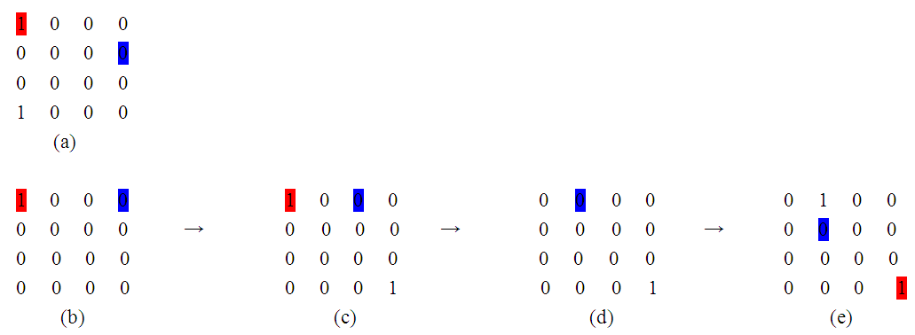 | Figure 5. Shows current state of EBDI-POMDP Agent and four perception steps in observer received from simple agents |
4.2.2. Experimental Results
As discussed above, often the optimal sensing policy is not affected by the sensing cost, as the sensing agents will send sensing information regardless of cost. Though, this not always so, hence to take sensing cost into account to evaluate EBDI-POMDP agent behaviour a new condition need to be added in this policy. For instance, if the request of sensing information maximises the EBDI-POMDP agent's deliberation utility, then it will be sent to agent otherwise end the process. Thus, the addition of this condition to the Boolean algebra function is shown in step 3 (Fig. 4), and can be solved by the use of observer layer with its own policy. This Simplify the evaluation task of the EBDI-POMDP agent's behaviour in varying sensing cost. Now, by using the same information in Table 1, and by supposing the planning and moving cost is one time unit and varying sensing cost q=0,1,2,4 time unit, we can plot the experimental results as in Fig. 6 which shows sensing cost effect in EBDI-POMDP agent behaviour in TILEWORLD. In Fig. 6 an EBDI-POMDP agent in varying sensing cost which explicit effected in its behaviour. So, cheapest sensing cost very important to provide EBDI-POMDP agent important information about the change in the world, especially, when intended hole disappears or new hole closer than intended hole is appear.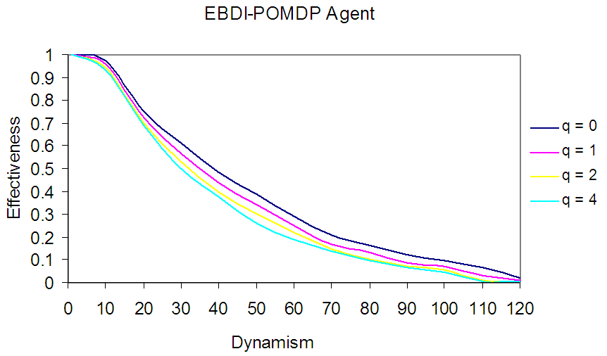 | Figure 6. An EBDI-POMDP Agent in varying sensing cost (q = 0, 1, 2 and 4) |
4.3. Dynamic Sensing Cost
Previous sections have shown that the sensing cost affects EBDI-POMDP agent behaviour in specific domain size with varying sensing cost, but we have supposed the sensing cost is static (constant) throughout a given experiment session. However, in reality the sensing cost may vary throughout a given trial. To study, this requirement, in this section we suppose that the sensing cost changes randomly over the grid, this means that the Boolean algebra function mentioned above will send sensing information if it is important and when sensing cost is within the cost interval  . Where
  is the minimum value of sensing cost and
  is the maximum value. In this experiment, a uniform distribution of sensing cost within [0, 4] interval. This means that the minimum value of sensing cost is zero and the maximum value is 4, with uniform probability distribution. Fig.7 shows EBDI-POMDP agent in TILEWORLD size 20×20 with one time unit of planning cost and sensing cost q changing randomly within [0, 4] interval. Fig.7, illustrates the EBDI-POMDP agent fluctuation due to random changing value of the sensing cost.
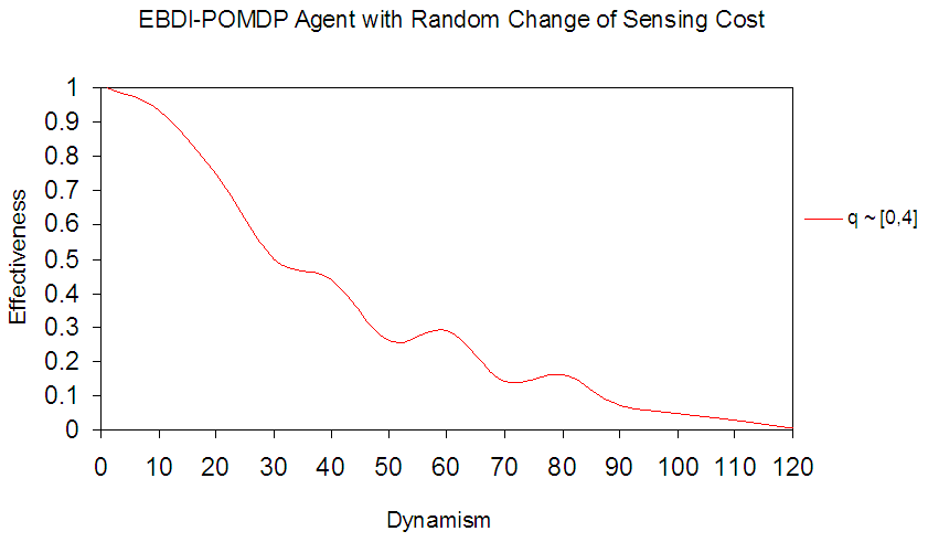 | Figure 7. Shows EBDI-POMDP Agent with one time unit of planning cost and random change of sensing cost (q ~ [0, 4]) |
4.4. Dynamic Planning Cost
This section deals with planning cost in the same way as the randomly changing sensing cost described in the previous section. Fig. 8, illustrates the fluctuation of the agent performance. The behavior of EBDI-POMDP agent in Fig.8 represents fluctuations among the agent's previous behaviors when planning cost value p fluctuates among 1, 2, and 4.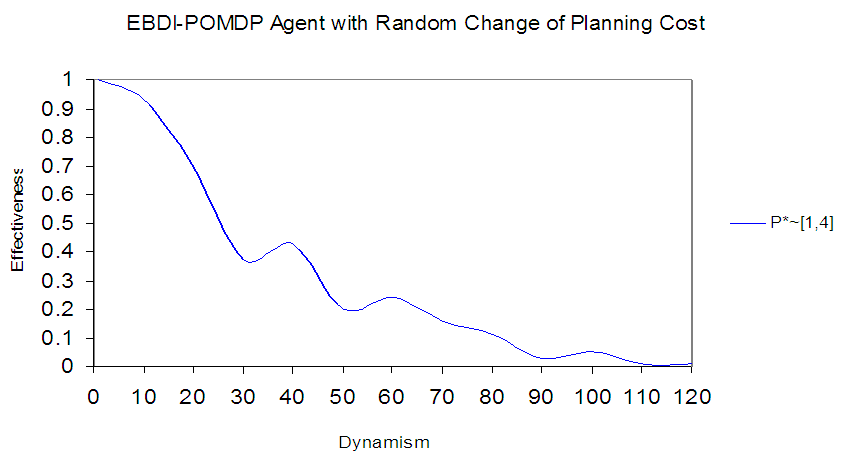 | Figure 8. Shows EBDI-POMDP Agent with one time unit of sensing cost and random change of planning cost (P* ~ [1, 4]) |
4.5. Increasing Size of World
This section tries to generalize the deliberative regulation policies and the associated mechanisms detailed in previous sections, in order to cope with the TILEWORLD size increase from 20×20 to 100×100. To this end, the experiment studies two aspects, namely: (i) the effect of the world size increases on sensing process, (ii) on planning process?
4.5.1. Effect on Sensing Process
This considers how one observer (filter) can control a big, dynamic and noisy area, especially, when sensing cost increases. The observer in this case will receive poor environment’s sensing information from simple agents. As when the TILEWORLD size increases the state space increases too. For instance, the state space in the 100×100 TILEWORLD case is 1002, whereas in the case of 20×20 the state space is equal to 202. This affects the planning complexity.Now, by using the same parameters of experiment in previous sections shown in Table (1) with the same number of obstacles but in average distance of world  and planning (moving) cost is one time unit, with varying sensing cost q. The experiment results shown in Fig. 9 show worse behaviour of EBDI-POMDP agent in TILEWORLD at all. Thus, to improve this behaviour we need many observers working together in multiple zone of the world. Each observer responsible of its zone and collaborates with other observers. So, if we divide the world to five zones, we need five observers to obtain the behavior of EBDI-POMDP agent in Fig. 6 in sect. 4.2.2.
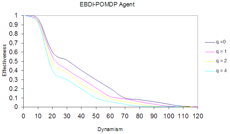 | Figure 9. Shows EBDI-POMDP Agent in 100×100 world size with varying sensing cost (q=0,1,2 and 4) |
Fig.10 illustrates the different EBDI-POMDP agent behaviours in varying sensing cost. Where the first three curves represent EBDI-POMDP agent in world size 20×20 and other three curves represent EBDI-POMDP agent in world size 100×100.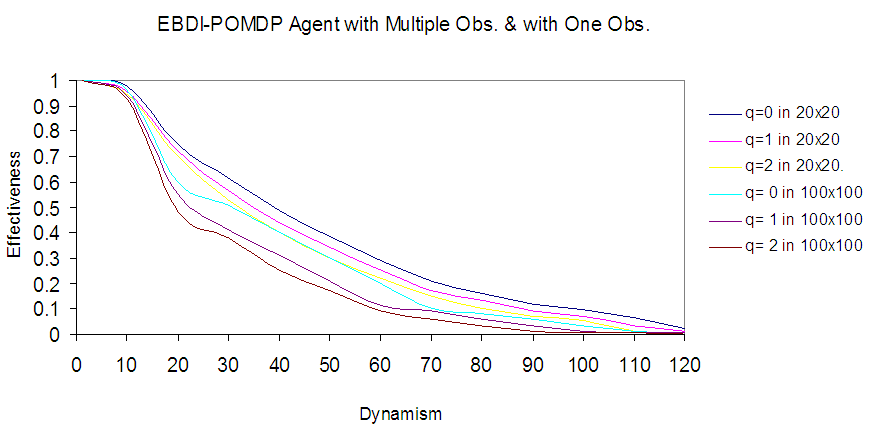 | Figure 10. Shows comparison between EBDI-POMDP Agent behaviors, the first three curves represent the agent world size 20×20 and the other three curves represent the agent in 100×100 world size, and varying sensing cost (q=0,1,2 and 4) |
4.5.2. Effect on Planning Process
Evidently, as argued above the use of one deliberative agent (EBDI-POMDP) will perform poorly when the world size increases to 100×100 especially when dynamism increases. However, it is possible to show EBDI-POMDP agent's behaviour in TILEWORLD size 100×100 with varying planning cost and one time unite of sensing cost for five observers in the world, each observer works in its zone (Fig. 11).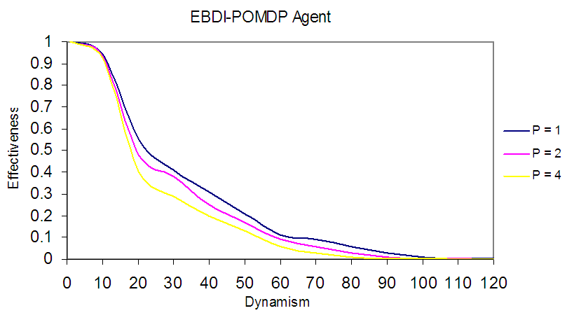 | Figure 11. Shows EBDI-POMDP Agent in 100×100 size of world with one time unit sensing cost and varying planning cost (p=1,2 & 4) |
The worse behaviour of EBDI-POMDP agent as shown in Fig. 11 reflects the huge and long deliberative tasks undertaken by agent especially when compounded by the increasing dynamism. In other words, to improve the deliberative agent’s performance to the level obtained in Fig. 2 when the TILEWORLD size was 20x20, one alternative solution is to use at least 5 collaborative deliberative agent for instance scanning a 20×20 partition of the 100x100 TILEWORLD. In Fig. 12, illustrates the behaviour of one EBDI-POMDP agent working in its 20×20 zone (partition), with varying planning cost p*=1, 2 and 4. Also, Fig. 12 shows the same results in Fig. 2 but with sensing cost one time unite, while in Fig. 2 was suppose sensing cost to be nil.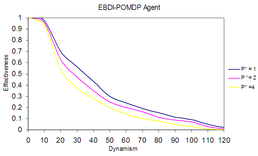 | Figure 12. Shows optimal behavior of EBDI-POMDP Agent in 20×20 world size with one time unit of sensing cost and varying planning cost (p*= 1, 2 and 4) |
Furthermore, a comparison between the agent performance shown in Fig. 11 and Fig.12 is presented in Fig. 13, in which the first three curves represent EBDI-POMDP agent as a part of five agents, each agent works in its 20×20 zone and others three curves represent EBDI-POMDP agent working alone in world size 100×100.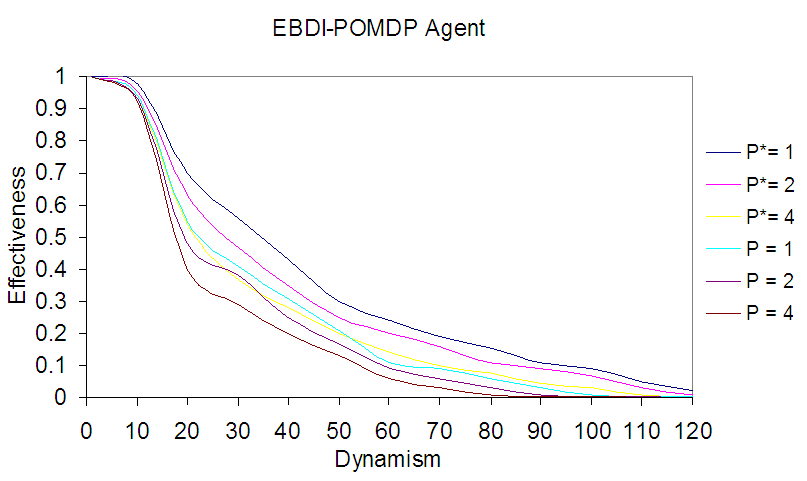 | Figure 13. Shows comparison between two deliberative agents, once embedded in its zone size 20×20 and the second in world size 100×100, with varying planning cost (p, p* =1,2 and 4) |
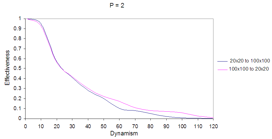
To study the EBDI-POMDP agent's performance if the world size vary randomly throughout a given experiment, the average distance of world d has been used to represent the mean distance of the world at any given time t. Where d value can be defined as  , that is, the average distance of world d ranges from 12 (average distance of world 20×20) to 60 (average distance of world 100×100). The other parameters are shown in Table (1). Fig. 14 and Fig. 15 show EBDI-POMDP agent performance in dynamic world size starting from 20×20 increasing to 100×100, when sensing cost q= 2 and planning cost p = 2 respectively.
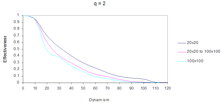 | Figure 14. Shows EBDI-POMDP Agent in multiple world size, the first curve represents the agent in 20×20, the second curve represents the agent in world starting from 20×20 increasing to 100×100, and the last curve represents the agent in 100×100, when sensing cost q = 2, and planning cost one time unit |
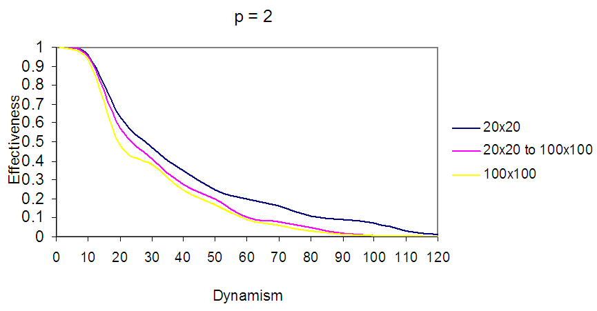 | Figure 15. Shows EBDI-POMDP Agent in multiple world size, the first curve represents the agent in 20×20, the second curve represents the agent in world starting from 20×20 increasing to 100×100, and the last curve represents the agent in 100×100, when planning cost p = 2, and sensing cost one time unit |
In Fig.14: Shows EBDI-POMDP Agent in multiple world size, the first curve represents the agent in 20×20, the second curve represents the agent in world starting from 20×20 increasing to 100×100, and the last curve represents the agent in 100×100, when sensing cost q = 2, and planning cost one time unit.In Fig. 15 the first curve represents the agent in world size 20×20 with planning cost p=2, the second curve represents EBDI-POMDP agent in world size starting from 20×20 increasing to 100×100 with planning cost p=2, and the last curve shows the agent in world size 100×100 when p=2, and sensing cost one time unit. In addition, it is possible to show EBDI-POMDP agent in world size starting from 100×100 decreasing to 20×20, Fig. 16 and Fig. 17 show these behaviours when sensing cost q=2 and planning cost p=2 respectively.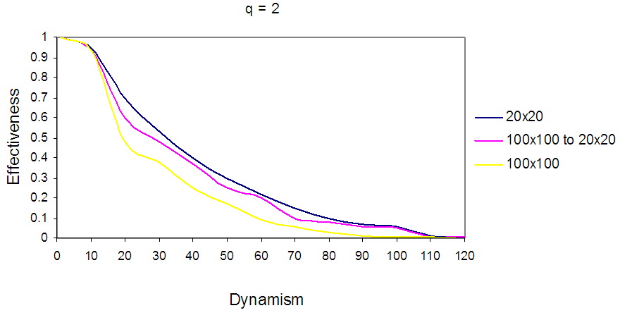 | Figure 16. Shows EBDI-POMDP Agent in multiple world size, the first curve represents the agent in 20×20, the second curve represents the agent in world starting from 100×100 decreasing to 20×20, and the last curve represents the agent in 100×100, when sensing cost q = 2, and planning cost one time unit |
 | Figure 17. Shows EBDI-POMDP Agent in multiple world size, the first curve represents the agent in 20×20, the second curve represents the agent in world starting from 100×100 decreasing to 20×20, and the last curve represents the agent in 100×100, when planning cost p = 2, and sensing cost one-time unit |
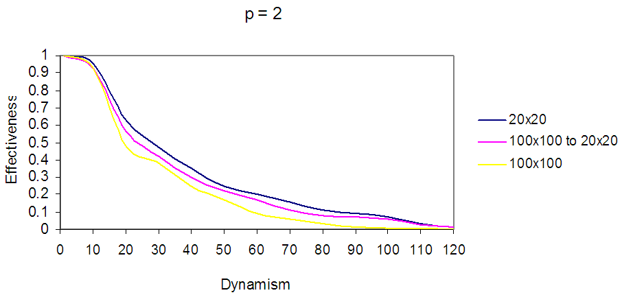
In Fig. 16 the first curve represents the agent in world size 20×20 with sensing cost q=2, the second curve represents EBDI-POMDP agent in world size starting from 100×100 decreasing to 20×20 with sensing cost q=2, and the last curve shows the agent in world size 100×100 when q=2, and planning cost one time unit.In Fig. 17 the first curve represents the agent in world size 20×20 with planning cost p=2, the second curve represents EBDI-POMDP agent in world size starting from 100×100 decreasing to 20×20 with planning cost p=2, and the last curve shows the agent in world size 100×100 when p=2, and sensing cost one time unit.Finally, an interesting comparison between EBDI-POMDP agent's behaviours in world size starting from 20×20 increasing to 100×100, and starting from 100×100 decreasing to 20×20, Fig. 18 and Fig. 19 show this comparison for sensing cost q=2 and planning cost p=2 respectively.In Fig. 18 and Fig. 19 the black curve represents EBDI-POMDP agent in world size starting from 20×20 increasing to 100×100, also it is started with higher effectiveness than red curve which represents EBDI-POMDP agent in world size starting from 100×100 decreasing to 20×20, but when dynamism increases and the world size starting to change the red curve outperforms the black curve.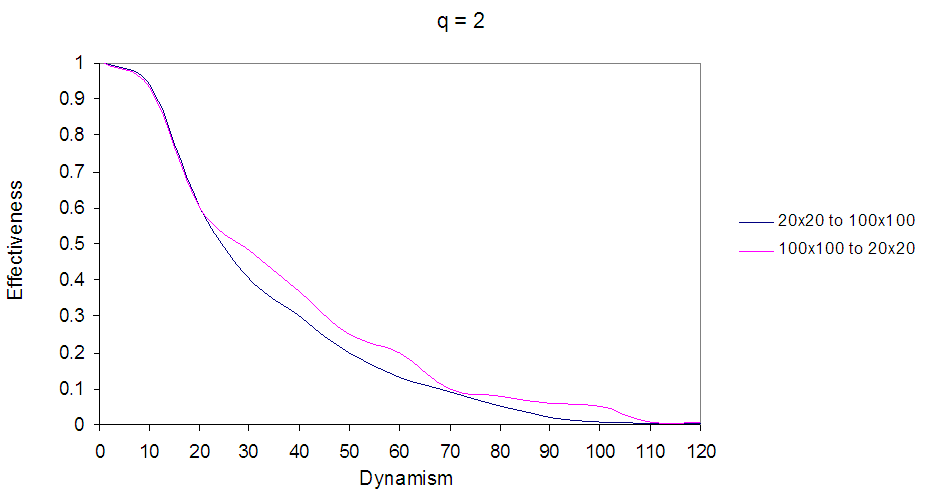 | Figure 18. Shows EBDI-POMDP Agent in multiple world size, the black curve represents the agent in world starting from 20×20 increasing to 100×100, the red curve represents the agent in world starting from 100×100 decreasing to 20×20, when sensing cost q = 2, and planning cost one time unit |
 | Figure 19. Shows EBDI-POMDP Agent in multiple world size, the black curve represents the agent in world starting from 20×20 increasing to 100×100, the red curve represents the agent in world starting from 100×100 decreasing to 20×20, when planning cost p = 2, and sensing cost one time unit |
4.6. Discussion
In this article, we extended the TILEWORLD experiments performed in [1], this extension used the self-organizing agent model to scan the environment and broadcast the event in accordance with a specified filtering and sensing policy set. This extension provided a general framework to enable the use of meta-layering and reasoning to improve the performance of EBDI-POMDP deliberative regulation taking into account changing world size, and planning, sensing and feedback (filtering) policies. This framework enables designers with a mathematical model to use hierarchical clustering and data aggregation and filtering to integrate knowledge-based and self-organizing system based regulation. For instance, as detailed in method described in this article:• First Layer: which contains a number of simple agents (even finite state automata) embedded in each node. This is for instance providing sensing information for a given hole (or even a composite TILEWORLD). • Middle layer: which filters the world sensing information received (or observed) from simple agents.• Second Layer: which uses the knowledge base model EBDI-POMDP agent and backward information as artificial immune system to determine the changes in specific properties, either represent a risk or benefit by the same diagnosing way which done in [1] but with decreasing the uncertainty which yields from combining self-organizing system to model. The optimal EBDI-POMDP policy lets the agent deliberate when a hole appears that is closer than the intended hole (but not on the path to the intended hole), and when the intended hole disappears. The experimental results have shown an overall improved agent deliberation performance compared to those obtained in [1]. In other words, the uncertainty decreased due to knowledge received from the sensing layer. However, in high dynamic domain the agent succeeds in filling those holes whose life-expectancy are sufficiently long, and even in highly dynamic world. There will be some holes that meet these criteria. Hence, the agent may success to fill only a small fraction of the holes.
5. Conclusions
Situated agents are artificial systems capable of intelligent, effective behaviour in dynamic and unpredictable environments. In this paper, we extended the TILEWORLD experiments performed earlier by Obied, Taleb and Randles in [1]; Interesting developments of EBDI-POMDP agent when dynamism increasing is integrate it with Self-Organizing system, to diagnose complex environment's changes to decrease the uncertainty. This article clear distinguishes between sensing policy and sensing cost, since; it described experiments examining the efficacy of dynamic sensing policy when the time cost of processing sensor information is significant. This paper demonstrates that several expected features of sensing cost and planning cost do arise in empirical tests. In particular, it is trying to answer the question is how would scalability of agent improve? The observations that for a given sensing cost and degree of world dynamism, an optimal sensing rate exists and, it is shows how this optimal rate is affected by changes in these parameters. The results indicate that and dynamic sensing policies with static and dynamic sensing and\or planning cost can be successful. Furthermore, it generalized the effects for larger world size, an important conclusion from above experiments the behavior of EBDI-POMDP agent improves if the number of agents increases in the same zone. Also, if the agent got started from specific world size which changes over the agent's trail to another world size (increases or decreases) the EBDI-POMDP agent still effective in varying dynamism. Moreover, to get sensing operation cheaper we need to change simple agents from full and fixed agents to agents do sensing by random search, which represents interesting future work for this article.
References
| [1] | A. Obied, A. Taleb-Bendiab, M. Randles. Self Regulation in Situated Agents. In Proceedings of 1st Intl, Workshop on Agent Technology and Autonomic Computing. Erfurt, Germany. Special Issue in ITSSA, V.1 N.3, 2006. p. 213-225. |
| [2] | D. Kinny, M. Georgeff and J Hendler, Experiments in Optimal Sensing for Situate Agents, Proceedings of the Second Pacific Rim International Conference on Artificial Intelligence, PRICAI '92, Seoul, Korea, July 1992. |
| [3] | M E Pollack and M Ringuette, Introducing the Tileworld: Experimentally evaluation Agent Architectures. In Proceedings of the 8th National Conference on Artificial Intelligence (AAAI-90), Boston, MA, 1990, pp. 183-189. |
| [4] | N L Badr, An Investigation into Autonomic Middleware Control Services to Support Distributed Self-Adaptive Software, PhD thesis, Liverpool John Moores University, UK, November 2003, pp. 60-75. |
| [5] | L Chrisman and R Simmons, Sensible Planning: Focusing perceptual attention, In Proceeding of 9th National conference on Artificial Intelligence, AAAI-91, Los Angeles, CA, 1991, p 756-761. |
| [6] | B Abramson, An analysis of error recovery and sensory integration for dynamic planners, In proceeding of 9th National conference on Artificial Intelligence, AAAI-91, Los Angeles, CA, 1991, p 744-749. |
| [7] | M E Bratman and D J Irsrael, and M E Pollack, Plans and Resource-Bounded Practical Reasoning, Computational Intelligence, Vol. 4, 1988, pp. 349-355. |
| [8] | R Bellman, Adaptive Control Processes: a Guided Tour, Princeton University Press, Vol. 2, 1961, pp. 30-55. |
| [9] | N Vlassis, A Concise Introduction to Multiagent Systems and Distributed AI, Intelligent Autonomous Systems Information Institute University of Amsterdam, 2003, pp 30-33. |
| [10] | A G Barto and R S Sutton, Reinforcement Learning: An Introduction, MIT Press, Cambridge MA, Vol. 1, 1998, pp. 30-75. |
| [11] | W Zhang, Algorithms for Partially Observable Markov Decision Processes, PhD thesis, The Hong Kong University of Sciences and Technology, Hong Kong, August 2001, pp 30-100. |
| [12] | Self-Organizing System (SOS): http://www.calresco.org/sos/sosfaq.htm#1.1, 26th of September 2017. |
| [13] | M Georgeff and D Kinny, Commitment and Effectiveness of Situated Agents, Proceedings of the 12th International Joint Conference on Artificial Intelligence (IJCAI-91), Sydney, Australia, April 1991, Morgan Kaufmann Publisher, pp. 82-88. |

 Abstract
 Reference
 Full-Text PDF
 Full-text HTML