1. Introduction

Microarray technology came on time to cover the need to monitor in parallel all the DNA sequences and to have the adequate sensibility to detect the variation of gene expression. There may be tens of thousands of spots on an array. Each spot contains tens of millions of identical DNA molecules with lengths from tens to hundreds of nucleotides. Afterwards, the microarray slide is exposed to a set of labeled cDNA samples, which are derived from tissue of interest. With the completion of hybridization reaction, the amount of the target that bounds to each sample is measured with the aid of image capturing devices and computer technology. The measurement is based on the intensity of the spot. There are three basic steps in the processing of microarray image [1]; gridding, segmentation, and quantification.

The first step is gridding; to assign coordinates to every element of the spot array. Gridding is the primary task of cDNA microarray image analysis; therefore it is a prerequisite for follow-up to microarray analysis.

Major work has been presented in the domain of microarray image gridding. Reference [2] described a semi-automatic system which mainly focused on the problem of finding an individual spot with high accuracy. Reference [3] introduced a technique using morphological operators to perform automatic gridding procedures for sub grids and spots. Reference [4] described a system for microarray gridding and quantitative analysis that imposed different kinds of restrictions on the print layout. That method required the rows and columns of all grids to be strictly aligned. Antoniol and Ceccarelli 2004 applied the markov random field approach which required the user’s input of the size of the spot, and the number of rows and columns. Reference [5] used a predefined image filter to grid the sub-array image.

During the recent years, there have been methods and software packages available that deal with one or a few of the aforementioned problems, such as ScanAlyze, 19 Spot (Buckly 2000), and GenePix Pro6 (Axon Instruments Inc. 2004). However, they all require a certain level of human intervention for achieving the desired accuracy, which imposes a big burden on the biologists who use microarrays in their research [6].

Image segmentation is the process of distinguishing objects from their background [7]. It is usually the first step in vision systems, and is the basis for further processing such as description or recognition. The goal of segmentation is to extract important features from images. Segmentation of an image can also be seen, in practice, as the classification of each image pixel to be assigned to one of the image compositions.

Different segmentation methods have been presented include the dynamic system modeling based approach [8] performs pixel clustering operations in a parallel manner to speed-up the segmentation process. The cellular neural network scheme [9, 10] segments the spots by performing a number of operations such as background clean-up, grid analysis, irregular spot elimination, and intensity analysis. The morphology based approach [11] uses a series of optional steps to segment the microarray image. The combination of Markov random field based grid segmentation and active contour modeling constitutes an approach suitable for spot detection and segmentation [12]. The two-stage clustering based approach [13] is comprised of spots boundaries adjusting and intensity-based partitioning operations. The use of adaptive thresholding and statistical intensity modeling is the base for some segmentation schemes [14], whereas another approach [15] uses a seeded region growing algorithm to identify spots of different shapes and sizes. Histogram and thresholding operations were used to classify microarray image samples into either foreground (spots) or background pixels [16].

One of the key steps in extracting information from a well gridded microarray image is the segmentation whose aim is to identify which pixels within an image represent which gene. This task is greatly complicated by noise within the image and a wide degree of variation in the values of the pixels belonging to a typical spot. An effective fully automated gridding technique followed by a comparison between four different segmentation methods is presented on a noisy microarray image, with high accuracy. The paper is organized as follows: a brief introduction is presented in this section, section 2 presents the used materials, section 3 summarizes the proposed gridding and segmentation methods for various cDNA microarray noisy images and section 4 discusses the results of the applied algorithms on microarray data set image. Conclusions are presented in section 5.

2. Materials

Different images have been selected from two different data sets, to test the performance of the proposed methods. They have different scanning resolutions, and different noise types, in order to study the flexibility of the proposed methods to detect spots with different sizes and features.

The images are stored in TIFF files with 16-bit gray level depth. A chosen microarray image with various kinds of artifacts or noises is drawn from Princeton University Microarray (PUMA) database [17].

The image includes thirty two sub-grids presenting acute lymphoblastic leukemia tissues (PUMA Experiment ID: 10223). The slide name is (shae082) and it is a cDNA microarrays spotted by a total of 24192 genes.

MATLAB [18] is used for data analysis and technical computing, as it is a high performance and powerful tool. MATLAB version is 7.11.0.584 (R2012b) on a windows 7 platform. The P.C used has a processor: Intel (R) Core (TM)i5 – 2.27 GHz. CPU with 2GB of memory.

3. Methods

3.1. Microarray Image Gridding

A gridding method using projection technique is proposed. This method is useful to eliminate various types of noise occurred in microarray images. Preprocessing microarray image is required before applying the gridding step, in order to remove noise which has gray values on the black background using Global Background Noise Correction. It can be implemented through a number of steps staring by getting the median intensity value of the image, then check each pixel value in the image, and compare this value with the obtained median value. If the pixel intensity value is less than the median value, we set it to zero. Otherwise, the pixel value is remained as shown in figure 1.

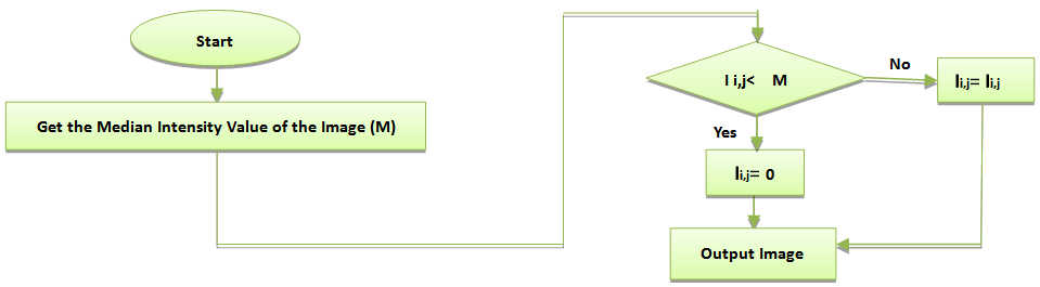Figure 1. Flowchart of Global Background Noise Correction

Where, I_i,j is the intensity value of the pixel in the row and the column. Because of the low-intensity features that are not well distinguishable from the background in most of the microarray images, it's important to develop a new method to improve the contrast between the foreground (spots) and the background using histogram equalization [18-20]. Unfortunately, an additive noise (small white spots) appeared on the background which can be eliminated using wiener filter [18-20]. In order to remove the large flare noise; at first the erosion operator with a structuring element (In experiment se = 7) is applied to remove foreground spots [18, 21], then apply image reconstruction to the result background [18, 19]. An image with less noise is obtained by subtracting resulted background from original image. This is mainly to remove large flare noise. After that, morphological opening with a structuring element (In experiment se = 4) is applied to remove small spikes in the image and at last apply image reconstruct again to the obtained image as shown in figure 2.

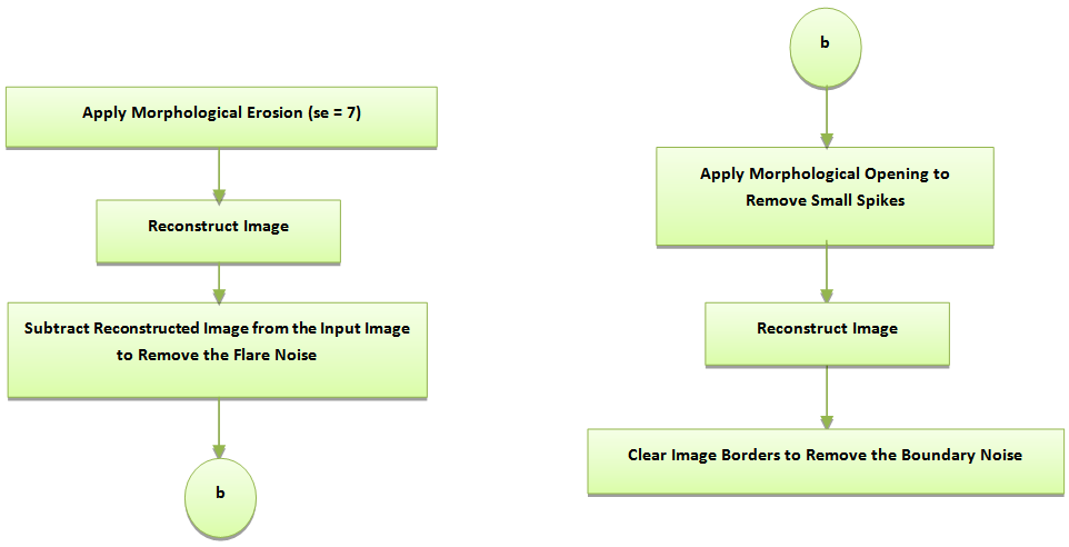Figure 2. Flowchart of Flare Noise Removal

The Projection Profile Method is then applied to the binary image obtained using canny edge detection operator [22, 23]. Then, the detected spots are filled using region filling operation. Despite canny detector is one of the best edge detectors that suppresses noise, it couldn't detect some spots well in the image, as it produces some incomplete regions which is difficult to be filled. To overcome this problem; morphological opening (erosion then dilation) is applied on the resulted binary image [21]. In order to obtain the horizontal intensity projection profile H P(y) of the image [24] f(x,y), the sum of intensity values are calculated at each pixel along the x-axis for each row, which is defined as follow:

(1)

Where, image size is X × Y, HP(y) represents the horizontal projection signal. The negative peaks of the profile are detected that correspond to the positions of the vertical grid lines. The actual image contains noise and other factors, so if directly use the above method for gridding, it may cause the phenomenon of missing or redundant grid lines. Therefore, to grid the image correctly, de-noising and refinement of the projection profile is required.

Finally, to determine the horizontal grid lines, the image matrix is transposed for only one time, and then repeats the previous steps starting from obtaining the projection profile. After all these steps it is found that There is a need to apply the Post- Processing Technique as there're a lot of sharp spikes may be appeared on the image profiles, that is treated as that false peaks. So, before performing the computations, a new approach is proposed to enhance and de-noise the calculated profile by applying two filters: un-sharpening and smoothing. The smoothing filter size value was set to 7 according to the experiment. The proposed method [25] has high accuracy, but in practice, no methods can grid entirely correct. Therefore, a grid correction or refinement method is developed through the following steps:

Ø Apply autocorrelation to the mean horizontal profile [18, 24], where, autocorrelation [26] is the cross-correlation of a signal with itself.

Ø Get the maximum peak indices from the auto correlated profile.

Ø Calculate an estimated period, which is a distance between two adjacent spot centers.

Ø By experiment, Compare between the obtained estimated period (E) and the distance between each two adjacent minimum peaks (M) obtained.

Ø When M < 0.5 E, there will be a mistakenly drawn line. Therefore, take a new index (inew) between the two adjacent minimum peak indices (i, i+1), where,

i_new = (i + (i+1)) /2.

Ø Then, the fault indices (i,i+1) are eliminated, and then,

i_new = i.

3.2. Segmentation

Once grids have been placed, discrimination between areas that are considered the spotsignal and areas that are considered the background signal must be carried out. The process, by which each individual cell in the grid must be selected to determine the spot signaland to estimate the background hybridization, is called segmentation. That information will be put towards a quantitative measurement at each cell. There are four presented approaches for segmentation; fixed circle segmentation, adaptive circle segmentation, thresholding segmentation, and adaptive shape segmentation.

• Fixed Circle Segmentation

Fixed circle segmentation method assigns all the spots the same size and shape. It uses a constant-diameter circle as the shape of all the spots in the image. The proposed fixed circle segmentation technique is presented as in the following steps:

1. Input the gridded image.

2. Get the region of interest (R.O.I.).

3. Let I = i^th row in the R.O.I.

I = 1 to end of R.O.I.

4. For each I, we calculate the center of its corresponding boundary box.

5. Draw a circle with the obtained center and the obtained estimated period (distance between two adjacent spots).

• Adaptive Circle Segmentation

Adaptive circle segmentation considers the shape of each spot as a circle, where the center and diameter of the circle are estimated for each spot. It involves two steps. First, the center of each spot needs to be estimated. Second, the diameter of the circle has to be adjusted. Adaptive Circle Segmentation method is shown in figure 3.

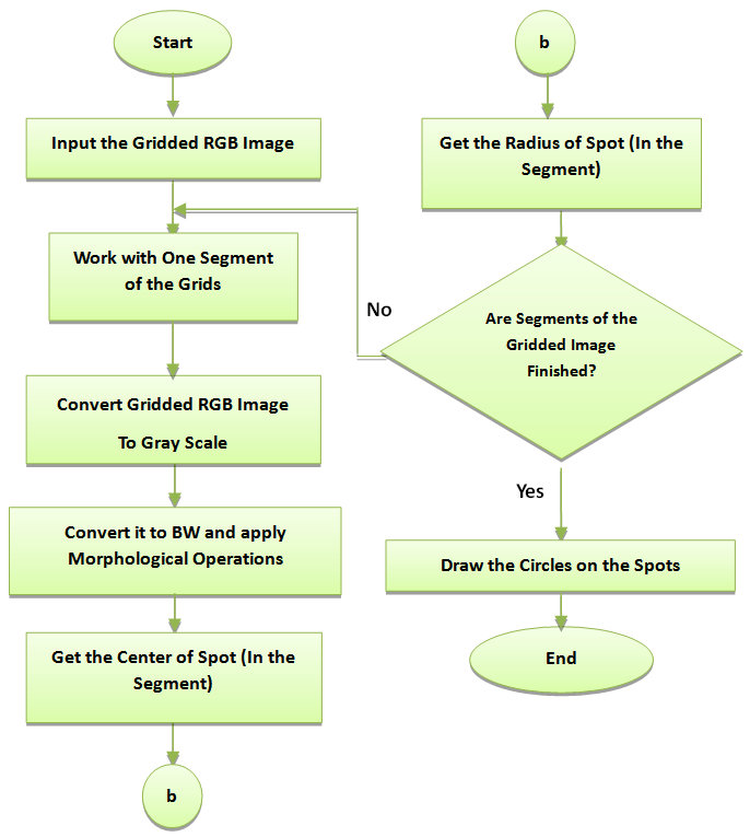Figure 3. Flowchart of Adaptive Circle Segmentation

• Thresholding Segmentation

The first step to start this technique is to apply a single threshold level to the whole image, so all spots are detected equally. However, it doesn’t work so well due to the large differences in the spot brightness. One way to equalize large variations in magnitude is by transforming intensity values to logarithmic space. This works much better, but some weak spots are still missed. Alternatively, the bounding boxes can be used to determine local threshold values for each spot. For an overview of the Thresholding segmentation algorithm the reader is referred to figure 4.

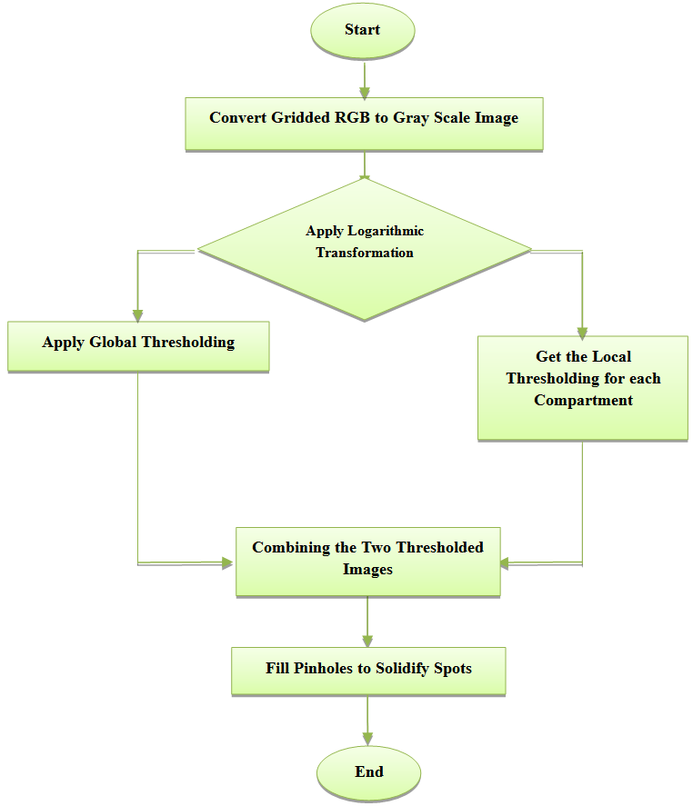Figure 4. Flowchart of Thresholding Segmentation

Unfortunately, results reveal that weak spots showed up well but spots with bright perimeters were as bad as the original global threshold before log space transformation. Since each of the local and the global thresholding has a special advantage, we combined the best of both approaches. These spot segmentation results were indeed much better.

The silhouettes of some spots still contained pinholes. The whole image could be filled using image filling operation, but this may not be a good idea. Notice that some spots run together. If four mutually adjacent spots (sharing a common corner) were all joined at their edges then a single function call would incorrectly fill in the common corner as well. To avoid that possibility, it is safer to fill each spot; take each bounding box region at a time by looping. Indeed, the spot segmentation now looks quite good [27].

• Adaptive Shape Segmentation

Seeded region growing (SRG) is a common technique that deals with different shapes in image segmentation. In SRG, the regions grow outwards from the seed points, preferentially, based on the difference between the pixel value and the running mean of values in an adjoining region. This method requires an initial point to be known, which is called the seed. After obtaining the seeds, the process is repeated simultaneously for both foreground and background regions until all the pixels are assigned to either foreground or background. Those pixels that are adjacent to a region are assigned first according to its intensity. Figure 5 shows the steps of applying the method.

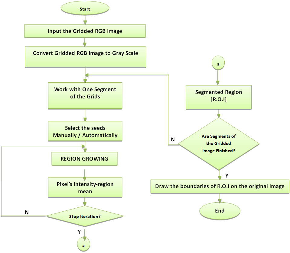Figure 5. Flowchart of S.R.G. Segmentation

An important advantage of SRG method is that it can be applied to microarray images containing spots of any shape and size.

The seed; which is the initial point to start applying the method is determined automatically. The pixel which has the maximum intensity in the spot window: as that point should most probably one pixel of the inspected spot.

4. Results and Discussion

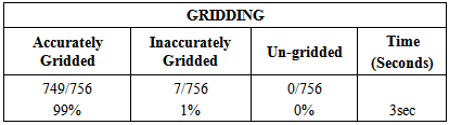
Anautomatic gridding method based on noise removal and four different segmentation methods; Fixed Circle, Adaptive Circle, Thresholding, and Adaptive Shape Segmentation were presented.

These presented methods are tested on a number of noisy microarray images drawn from Princeton University Microarray (PUMA) database. The results of applying these segmentation methods on a microarray image are shown in this section. The chosen noisy microarray image includes thirty two sub-grids (PUMA Experiment ID: 10223) and it is spotted by a total of 24192 genes. To test the efficiency of the proposed methods, a sub-array in the fourth row and the second column was cropped as shown in figure 6.

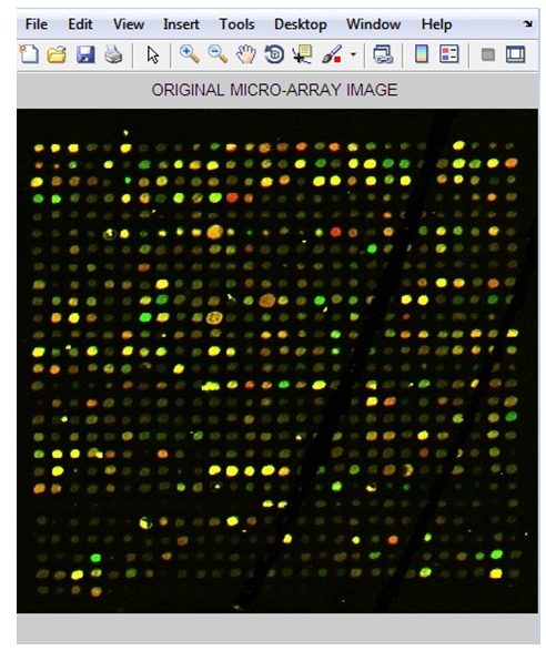Figure 6. The Original Microarray Image

4.1. Gridding

Figure 7 shows the detailed results after applying the proposed gridding method.

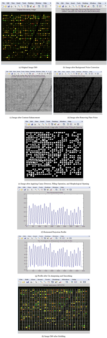Figure 7. Steps of applying the proposed gridding technique on original image

The accuracy (A) of the developed gridding method [28] on a specified input image, having N_{Total Spots}, can be calculated as:

(2)

Where, N_{Correct Spots}, N_{Total Spots} indicates the number of spots correctly gridded and the total number of spots in the image respectively.

As shown in table 1, the proposed method has higher accuracy, but in practice, no method can grid entirely correct. Therefore, pre-processing, post-processing, and refinement steps used, effectively enhance the contrast and eliminate various kinds of noise in the image. This applicable method can correctly grid the two selected types of microarray images without any human intervention. By comparing the proposed gridding method with other existing methods as those implemented by Deepa J and Tessamma Thomas [29], Basim Alhadidi [30], and Fatma El-ZahraaLabib [31], it was found that this method is more accurate and can grid various types of noisy images correctly as it mainly deals with noisy images.

Table 1. Results of Gridding Method

4.2. Segmentation

• Fixed Circle Segmentation

It was obviously shown that the fixed circle method clearly cannot satisfy the needs. Figure 8 shows the resulting image after applying the fixed circle approach. We can see that some regions within the high intensity areas (spots) are left out of the foreground, and some regions within the low intensity areas (background) are included in the foreground regions. That is because of the fixed diameter of all the drawn circles despite the variation in the diameters of the spots in the same image.

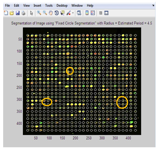Figure 8. Image after Applying “Fixed Circle Segmentation” Method

• Adaptive Circle Segmentation

The adaptive circle segmentation method achieves better results for circle-shaped spots. However, the spots in a microarray image can take shapes including ellipses. That is the main drawback of the adaptive circle segmentation method is that it restricts the shape, it’s obvious in figure 9.

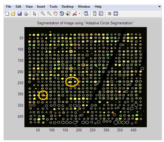Figure 9. Image after Applying “Adaptive Circle Segmentation” Method

• Thresholding Segmentation

Figure 10 shows the results of applying thresholding segmentation on the microarray image. It is clearly observed that when using the current segmentation method to separate background from foreground in microarray images, it gives good results in the images that have clear spots. But it cannot deal well enough with weak spots.

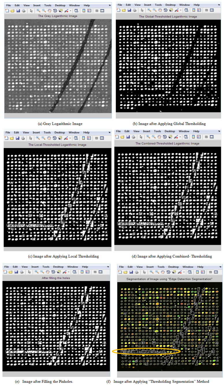Figure 10. Steps of applying “Thresholding Segmentation” technique on original image

• Adaptive Shape Segmentation

Figure 11 shows the result of applying the adaptive shape segmentation method using a maximum seed point. This method requires an initial point to be known, which is called the seed. An advantage of using SRG in microarray image segmentation is that the location of foreground pixels and background pixels can be estimated. It also deals with different shapes and sizes of spots.

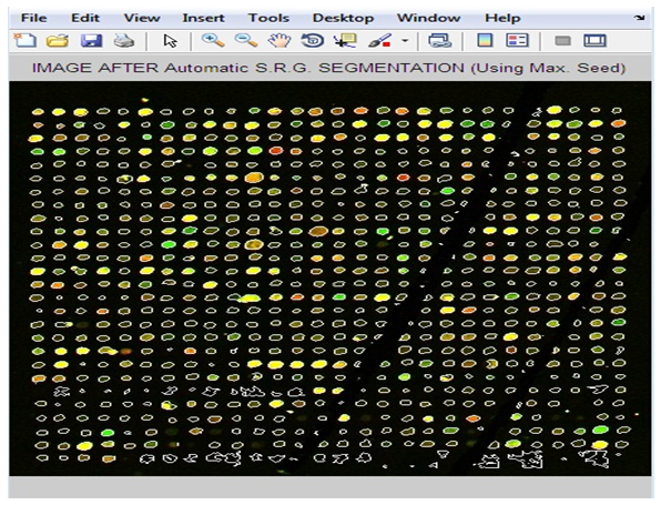Figure 11. Image after Applying “Adaptive Shape Segmentation” Method

The accuracy of the proposed methods was analyzed by means of a statistical analysis. More precisely, using the proposed approach, 91.5% of spots were “very efficiently segmented”, and no spurious spot were detected. A spot was “very efficiently segmented” if at least 90% of the entirespot area was enclosed in the contour of that spot [32]. By comparing the results of applying the four presented segmentation methods; Fixed Circle Segmentation, Adaptive Circle Segmentation, Thresholding Segmentation, Adaptive Shape Segmentation methods, It is clearly obvious that the Adaptive Shape Segmentation method can segment noisy microarray images correctly despite of the degree of noise and the shape and size of the spots. That is shown in table 2.

Table 2. Comparison between the Four Proposed Segmentation Methods

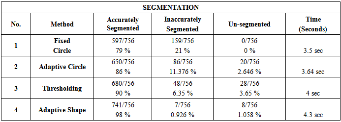
5. Conclusions

The development of biomedical research has been led by the increasing knowledge as well as new advances in technology. Traditionally, researchers were able to investigate a small number of genes at a time by using the available techniques back then. DNA microarray technology has enabled biologists to study all the genes within an entire organism to obtain a global view of genes’ interaction and regulation. This technology has a great potential in obtaining a deep understanding of the functional organization of cells. The emergence of this technology allows the researchers to tackle difficult problems and reveal promising solutions in many fields.

In this respect, our research based heavily on the requirement for areliable yet time efficient automated method. One of the key steps in extracting information from a well-gridded microarray image is the segmentation whose aim is to identify which pixels within an image represent which gene. This task is greatly complicated by noise within the image and a wide degree of variation in the values of the pixels belonging to a typical spot.

This work emphasizes the impact of well-gridded microarray image segmentation. The proposed gridding method depends on projection and applicable to various types of noisy microarray images. It gives very good results with accuracy 99%. In the segmentation stage, four segmentation methods have been presented; “fixed circle segmentation”, “adaptive circle segmentation”, “thresholding segmentation”, and “adaptive shape segmentation” methods. When the four proposed methods sere compared, it was found that the first two methods are shape-based segmentation methods. Fixed circle segmentation cannot segment clearly all types of images; when the spots size varies in the image, it will work badly. While the adaptive circle segmentation method achieves better results for circle-shaped spots. The other two segmentation methods; “adaptive shape segmentation” and “thresholding segmentation” gives better results. When using “thresholding segmentation” to separate background from foreground in microarray images, the current methods cannot deal well enough with weak spots. So, it was very clear that “adaptive shape segmentation” gives better results using a maximum seed with accuracy 98%.