1. Introduction

The road traffic simulation is an important tool for analysis and control of road traffic networks. However, a detailed simulation of very large networks (e.g. an entire city and larger) is still problematic due the computational and time requirements. In order to be able to simulate these networks in a reasonable time, the simulation can be adapted for distributed computing environment where combined power of multiple interconnected computers is utilized. During the adaptation of the simulation, it is necessary to divide the traffic network into sub-networks, which are then simulated on particular computers (nodes) of the distributed computer. The load-balancing of the sub-networks and the communication among them are two key issues of the distributed road traffic simulation.

In this paper, the performance of several methods for road traffic network division, which we developed, is compared. All the methods are focused on load balancing of the sub-networks and can be divided into two steps – assigning weights to the traffic lanes and their marking for division. The description of various approaches to these two steps, their combination and testing are the main contribution of this paper.

2. Distributed Road Traffic Simulation

The methods for traffic network division, which we developed, are intended for distributed discrete microscopic simulation of road traffic. Generally, the methods utilize various types of less-detailed simulation for assigning of the weights to the traffic lanes. For better understanding, the key aspects and issues of the road traffic simulation are described in following sections.

2.1. Simulation Types

There are several types of road traffic simulation, which can be divided based on the level of detail as microscopic, mesoscopic, and macroscopic simulation.

In a microscopic simulation, every single vehicle is considered with its own position, direction, speed, and acceleration. The vast majority of microscopic simulators use the time-stepped time-flow mechanism. This means that the entire simulation time is subdivided into sequence of equally-sized time steps. In each time step, the entire simulation state (i.e. positions of the vehicles) is recomputed [1]. The steps are usually one second long [2], [3]. The utilization of the time-stepped time-flow mechanism is relatively unusual from the point of view of a general discrete simulation, in which an event-driven time-flow mechanism (division of simulation time into sequence of time-stamped events) is usually employed. Due to high detail, the microscopic simulations are very computation-intensive, especially for large traffic networks.

The opposite side of the traffic simulation spectrum is represented by the macroscopic simulation, which deals only with aggregate traffic flows in particular roads or traffic lanes. The traffic flows are usually described by set of periodically recalculated parameters (e.g. mean speed and traffic density). These models are the oldest ones [4] and exist in many variations. Because there are no individual vehicles, the macroscopic models are far less computation-consuming than their microscopic counterparts.

The mesoscopic simulation fills the gap between the macroscopic and macroscopic simulations. There is a number of various traffic models, which falls in the realm of mesoscopic simulation, such as gas kinetic models [5] or queuing networks [6]. Both time-flow mechanisms are commonly used. Characteristics common to the majority of mesoscopic simulations are the description of traffic entities at high and their interactions at low level of detail [7]. Hence, a mesoscopic simulation can be much faster then a microscopic simulation, although individual vehicles often exist in the simulation in some form.

2.2. Simulation Decomposition

The division of the simulated traffic network into sub-networks represents a spatial decomposition of the simulation. Using this approach, the entire traffic network is divided into required number of parts (traffic sub-networks), which are then simulated by simulation processes running on the particular nodes of the distributed computer. It is the most common approach in the field of road traffic simulation. However, there are also other approaches, such as task parallelization and temporal decomposition. Their use in the field of traffic simulation is rare, but some examples can be found.

The task parallelization divides the simulation program into modules, which are then running on the particular nodes of the distributed computer. In order to maximize the efficiency of the distributed simulation, each module should consume similar amount of computational power [8]. However, this is problematic in the field of traffic simulation, because the major part of the computational power is consumed by the movement of the vehicles and collection of the statistical data. Hence, the task parallelization is used only in special cases of road traffic simulation (e.g. in [9]).

The temporal decomposition divides the simulation time into intervals, which are then simulated by the simulation processes on particular nodes of the distributed computer. So, each process simulates entire simulation (i.e. entire traffic network in case of road traffic simulation) but only for one time interval. The main disadvantage of this approach is that the states on the boundaries of the intervals may not match, especially in case of road traffic simulation, whose states are very complex. Nevertheless, an attempt to bring the temporal decomposition to the field of road traffic simulation can be found in [10].

2.3. Inter-process Communication

In the reminder of the text, only the spatial decomposition (i.e. division of traffic network into required number of sub-networks) will be considered.

Although the traffic network is divided, the resulting sub-networks should remain interconnected by set of traffic lanes. However each sub-network is restricted by the process, which performs its simulation. To ensure passing of vehicles in the connecting lanes, the processes must communicate each other [11]. So, the vehicles are transferred in the form of messages among the simulation processes [12].

In order to maintain the consistency of the simulation, all processes must perform the same time step at the same moment. Otherwise a causality error (i.e. arrival of a vehicle in an incorrect time step) can occur [1]. This is ensured by synchronization of the processes, which requires additional messages to be sent. Both the transfer of vehicles and the synchronization of the simulation are ensured by a communication protocol.

2.4. Microscopic Road Traffic Simulator for Testing

The developed methods for division of road traffic network, which will be described later in the text (see Section 4 and Section 5), were tested using the Distributed Urban Traffic Simulator (DUTS) developed at Department of Computer Science and Engineering of University of West Bohemia (DSCE UWB).

The DUTS system is a discrete microscopic time step simulator of urban traffic, which is able to be preformed on a single-processor or on a distributed computer [11].

3. Traffic Network Division Approaches

Now, as we discussed the issues of the distributed road traffic simulation, we can focus on the division of the road traffic network. The division method should consider two issues – the resulting load of the sub-networks and the resulting inter-process communication. The load-balancing of the sub-networks is important for similar speed of the simulation processes, because the slowest process slows down the entire simulation (due to the synchronization). The minimal inter-process communication is important, because it is much slower than the reminder of the simulation’s computations. Hence, an intensive inter-process communication can significantly affect the resulting performance of the distributed simulation [13].

The existing approaches to the traffic network division are usually focused on first or second issue, but can be also focused on both or neither. The issues are usually not considered during the traffic network division if the implementation of the distributed simulator is focused on solving of other issues, such as in [14]. However, a convenient traffic network division can significantly influence the resulting speed of the distributed road traffic simulation (see Section 6.2)

The examples of traffic network division are described in following sections.

3.1. Division into Equally-sized Rectangular Pieces

The division into geographically equally-sized pieces is the easiest solution, which neglect any optimization. An example of this approach can be found in the ParamGrid simulator [15], where the traffic network is divided into grid of rectangular pieces. This allows the simulation to be watched on a grid of displays. Each display is connected to one node of the distributed computer [15]. So, with proper hardware equipment, it is possible to watch the simulation of large areas online.

The main disadvantage of this approach is that the densities of traffic lanes in particular rectangular pieces and traffic density in the lanes are not considered [12]. Hence, the number of vehicles in various rectangular pieces can be very different, which can lead to slow down of the simulation. Also, the number of divided traffic lanes is not considered. This can lead to a very intensive inter-process communication [13]. Nevertheless, this approach is utilizable for traffic networks where the traffic lane density and traffic densities in the lanes are more or less uniform [12].

3.2. Minimization of Neighbours Count

A more advanced approach can be found in the TRANSIMS simulator [2]. This approach is focused on minimization of the neighbours count and divided traffic lanes count using graph partitioning methods (e.g. orthogo- nal recursive bisection). Nevertheless, the load-balancing of the resulting sub-networks is also partially considered, since the traffic network is divided into sub-networks of similar size. This size is calculated as the accumulative length of the lanes in the sub-networks [2].

The size of the traffic network, as defined in this method, can be problematic, because the traffic densities in the lanes are neglected. So, if there were very different traffic densities in various traffic lanes, the numbers of vehicles in the resulting sub-networks would be unbalanced [11]. This would lead to different speeds of the simulation processes and thus to slow down of the entire distributed simulation.

3.3. Load-balancing of Sub-networks during Division

The issue mentioned in previous section is solved in the UMTSS simulator [16]. Similar to the TRANSIMS simulator, a recursive bisection method is used for traffic network division. However, besides the length of the traffic lanes, the vehicle density in the lanes is also considered. The information of the vehicle density in the traffic lanes is estimated using the drivers’ route choice decision and the origin-destination matrix [16].

Another approach, which is focused on load-balancing of the resulting traffic sub-networks, can be found in the vsim simulator [3]. There, the division is performed using the numbers of vehicles moving within the particular traffic lanes of the divided traffic network. These weights of the traffic lanes are collected during one sequential simulation run [3]. This enables a division into load-balanced sub-networks for distributed simulation runs. It is a static load-balancing, since it is performed only once.

The main problem of this approach is the collection of the numbers of vehicles. If the simulation is intended to be distributed (the very reason for the division of traffic network), its sequential simulation run can be difficult to perform due to memory and time requirements [11]. Also, the number of divided traffic lanes is not considered during the traffic network division.

3.4. Load-balancing of Sub-networks during Simulation

A different approach to load-balancing of the sub-networks is to perform the traffic network division repeatedly directly during the simulation run rather than prior it. So, the division can be adapted based on the current load of the particular traffic sub-networks.

This dynamic load-balancing is utilized for example in [17]. There, the simulation run is divided into time intervals. The simulation is controlled by a master process and performed by the working processes. At the beginning of every time interval, the traffic network is divided using the prediction of the load of the particular traffic crossroads based on the load in the previous time interval. This division is performed sequentially by the master process and the resulting sub-networks are assigned to the working processes [17]. So, in every time interval, the traffic sub-networks are load-balanced.

4. Methods for Weights Assigning

Although the dynamic load-balancing of the traffic sub-networks ensures optimal division during the entire simulation run (see Section 3.4), it has also a non-negligible overhead. This overhead is caused by the repeated traffic network division directly during the simulation run. This means not only additional computations performed usually sequentially by a central master process [17], but also additional inter-process communication, since the updates of the traffic network division must be delivered to the particular simulation processes.

For the reasons mentioned in previous paragraph, we have decided to focus on static load-balancing of the resulting traffic sub-networks. The traffic network division method used in the vsim simulator (see Section 3.3) has an issue regarding the difficult collection of the numbers of vehicles in traffic lanes. However, it offers a good load-balancing of the resulting traffic sub-networks, because the division is based on the data acquired directly from the simulation. Hence, it served as an inspiration for the traffic network division methods, which we developed. Their general idea is to use a less-detailed simulation for assigning of the weights to the traffic lanes in a reasonable time. Using these weights, the traffic network can be divided into load-balanced sub-networks.

So, the process of traffic network division consists of two separate phases – the assigning of the weights to the traffic lanes (WA) and the marking of traffic lanes, which will be eventually divided (MTL). Originally, we developed three methods for traffic network division where each method utilized a different simulation for assigning of the weights and a different algorithm for marking of traffic lanes. However, since the two phases are separate, the methods were reconstructed and it is now possible to select the first and the second phase separately and combine various approaches.

Three methods for assigning of the weights to the traffic lanes are described in the reminder of this section. Two methods for marking of traffic lanes are described in Section 5. All methods are implemented in the DUTS Editor, a system for design and division of traffic networks for the DUTS system. Similar to the DUTS system, the DUTS Editor was developed at DSCE UWB.

4.1. Macroscopic-simulation-based Weights Assigning

The Macroscopic-simulation-based weights assigning (MaSBWA) method utilizes a macroscopic simulation. The vehicle density of the traffic flows in particular traffic lanes are used for calculation of the traffic lanes’ weights. The macroscopic simulation utilized in the MaSBWA method is inspired by the macro-JUTS model designed for the hybrid traffic model of the JUTS (Java Urban Traffic Simulator) system [18], which was also developed at DSCE UWB.

In the simulation, each traffic lane is divided into small segments (S) of the same size (Δx). Each segment has its own parameters of the traffic flow – the mean speed (v) and the vehicle density (ρ). The parameters of each segment are recalculated once per time step, whose length is preset to 2 seconds of the simulation time. The parameters of each segment are calculated using the parameters of the preceding segment (see Figure 1) [11].

Figure 1. Traffic lane in the macroscopic simulation

The crossroads are constructed as probabilistic division segments, no crossroad dynamic is simulated. Each crossroad consists of set of entries (E) and set of exits (X) connected to incoming (I) and outgoing (O) traffic lanes, respectively. The values of the parameters of the entries are calculated based on the parameters of the last segment of the lane, which is connected to the entry. The values of the parameters of the exits are calculated based on the values of the corresponding entries and the branching probabilities (p) (see Figure 2) [11]. If there are traffic lights, only the entries with green period are considered.

Figure 2. Traffic crossroad in the macroscopic simulation

The parameters of traffic flows incoming to the simulated area are generated using generators, which can produce deterministic traffic flows or stochastic traffic flows with exponential distribution. Depending on the flows, the entire simulation can be either deterministic or stochastic with exponential distribution [11].

Using the macroscopic simulation, each traffic lane can be assigned by a weight, which is calculated as the average sum of vehicle densities in all segments of the lane. The weight w_i of the ith lane can be calculated as:where R is the number of simulation runs, N is the number of steps of one simulation run, n_i is the number of segments of the ith lane and ρ_ijkl is the vehicle density in the jth segment of the ith lane in the kth time step of the lth run.

If the simulation is deterministic, one simulation run is sufficient for calculation of the weights, since all simulation runs are identical. If the simulation is stochastic, several simulation runs are required to ensure fidelity of the calcu- lated weights. Nevertheless, it has been determined that the deterministic simulation gives the same or even better results than the stochastic simulation. Contemporary, it is much faster [19]. Hence, the deterministic simulation is used in the MaSBWA method. For more detailed description, see [11].

4.2. Mesoscopic-simulation-based Weights Assigning

The Mesoscopic-simulation-based weights assigning (MeSBWA) method utilizes a mesoscopic simulation, which is based on a simple Nagel-Schreckenberg’s cellular automaton for freeway traffic [20].

In the simulation, each traffic lane consists of equally-sized traffic cells. The cells are 7.5 meter long and can be either empty or occupied by a single vehicle [20]. Each vehicle is represented as an integer value expressing its current speed (see Figure 3).

Figure 3. Traffic lane in the mesoscopic simulation

The speeds of the vehicles are expressed in cells per time step (c/ts). They are recalculated and the vehicles’ positions accordingly shifted once per time step using four basic rules – acceleration, deceleration, randomization, and movement. The first three rules ensure the acceleration of the vehicle to the maximal speed, the deceleration if there is an obstacle in the way (e.g. a slower vehicle), and a random deceleration in order to simulate the natural fluctuation of the speed. The last rule only shifts the vehicles in the lane accordingly [19].

The crossroads are constructed as routers of vehicles from the incoming to the target outgoing traffic lanes. The target traffic lane for a vehicle is determined using the possible travel direction, branching probability, and pseudo-random number generators. The passing of the vehicles through the crossroad is not modelled. However, the right of way and the information about the main road are used for ordering of the vehicles. Moreover, the vehicles are not allowed to pass the crossroad until there is a free cell in the target outgoing traffic lane (see Figure 4) [19]. Traffic lights are also modelled if necessary.

Figure 4. Traffic crossroad in the mesoscopic simulation

The vehicles incoming to the simulated area are generated using generators, which produce stochastic traffic flows with exponential distribution. So, the entire simulation is stochastic [19]. Unlike the MaSBWA method, a deterministic version is not implemented.

Using the mesoscopic simulation, each traffic lane is assigned by a weight calculated as the mean number of vehicles moving within the lane during the simulation run. The weight w_i of the ith lane can be calculated as:

(2)

where R is the number of simulation runs, N is the number of steps of one simulation run, and V_ijk is the number of vehicles in ith traffic lane in jth time step of the kth simulation run.

Due to the stochastic nature of the MeSBWA simulation, it is necessary to perform several simulation runs to ensure fidelity of the calculated weights. Based on the performed tests, it has been determined that the utilization of ten simulation runs offers sufficient fidelity for the traffic network division purposes. For more details, see [19].

4.3. Microscopic-simulation-based Weights Assigning

The Microscopic-simulation-based weights assigning (MiSBWA) method utilizes directly the microscopic simulation of the DUTS system. So, the microscopic simulation is not implemented in the DUTS Editor. Instead, the statistics of the number of vehicles moving within the traffic lanes in a simulation run are stored to a XML file, which can be then loaded by the DUTS Editor as the data source for the MiSBWA method. Hence, this method is very similar to the method used in the vsim simulator [3] (see Section 3.3).

Using the data from the microscopic simulation, the weights are calculated similar to the MeSBWA method (the same equation is used – see Equation (2)). Also, it is necessary to perform several simulation runs to guarantee the fidelity of the calculated weights. Again, similar to the MeSBWA method, ten simulation runs are commonly used. For more information, see [21].

5. Methods for Traffic Lanes Marking

Now, as we briefly described the methods for assigning weights to traffic lanes, we can proceed with the methods for marking of traffic lanes, which shall be divided. We have developed two methods, which employ a modified breadth-first search or a genetic algorithm.

The input of both methods is the traffic network with traffic lanes assigned by weights using any of the weight assigning methods (see Section 4). Both methods are described in following sections.

5.1. Modified Breadth-First Search

The Modified breath-first search marking of traffic lanes (MBFSMTL) method employs a modification of a standard breadth-first searching algorithm for graph exploration [22] for division of the road traffic network. Its primary objective is to create load-balanced sub-networks. However, the number of divided traffic lanes is also considered.

The MBFSMTL method starts with the calculation of the sum of all weights of the traffic lanes (total weight). Based on this total weight and the required number of sub-networks, the total weight per sub-network can be easily calculated. With these two values, it is possible to proceed with modified breadth-first searching of the traffic network, which is considered as a weighted graph for this purpose. The crossroads are the nodes and the sets of lanes connecting the neighbouring crossroads are the weighted edges (see Figure 5) [11].

Figure 5. Traffic network as weighted graph

At the beginning, a crossroad is selected as the starting node of the breadth-first search algorithm. This crossroad is assigned by the current sub-network ID, which is zero at this point. As the breadth-first search is performed, more and more nodes are becoming explored and assigned by the current sub-network ID. Also, the weights of all lanes neighbouring to the explored crossroad are added to the current sub-network’s current weight. When this value reaches the total weight per sub-network, the current sub-network ID is incremented and the current sub-network’s current weight is set to zero. This repeats until all crossroads are explored.

Once all crossroads are assigned by the sub-network IDs, the marking of traffic lanes is easy. It is sufficient to mark the lanes connecting crossroads with different IDs [11]. The entire algorithm is described using pseudocode in Figure 6.

Figure 6. Pseudocode of the MBFSMTL algorithm

5.2. Genetic Algorithm

The Genetic algorithm marking of traffic lanes (GAMTL) method employs a standard genetic algorithm [23] for a multi-objective division of the traffic network. The two objectives are the minimal number of divided traffic lanes and the load-balancing of the sub-networks.

Genetic algorithms are generally convenient for the multi-objective optimization problems [24]. They mimic the natural genetic evolution and selection in nature. This means that a single solution of a problem (an individual) is represented as a vector of boolean or integer values. An initial set of the individuals (initial population) is most often randomly generated. The individuals are then crossed and mutated in order to produce a new population. A fitness function is then calculated for each individual and the individuals with best fitness are selected to be parents of the next population [25]. The entire process repeats until a stop condition is fulfilled or a preset number of iteration is reached [25].

The GAMTL method assigns the crossroads to the particular sub-networks, similar to the MBFSMTL method (see previous section). Hence, an individual is represented by a vector of integers with length corresponding to the total number of crossroads (K). Each integer then represents the assigning of the corresponding crossroad to the sub-network and the maximal value at any index of the vector corresponds to the number of required sub-networks (M) (see Figure 7).

Figure 7. Representation of an individual

The initial population is randomly generated, which means that, in each individual, the crossroads are randomly assigned to particular traffic sub-networks. Using the fitness function, crossover, and mutation, the assignment of the crossroads in the individuals changes toward a solution where the sub-networks are load-balanced (based on the weights of the traffic lanes) and the number of divided traffic lanes is minimal [26].

The fitness function is used for objective assessment of each individual. It consists of two parts – the equability, which represents the load-balancing of the sub-networks, and the compactness, which represents the minimal number of traffic lanes.

The equability of an individual can be calculated using the total weights of the particular sub-networks as:

(3)

where E is the equability of an individual, is the mean total weight of one sub-network, w_Si is the total weight of the ith sub-network, and M is the number of sub-networks. The total weight of the ith sub-network w_Si can be calculated using the weights of the traffic lanes and the assignment of the crossroads to the sub-networks from the individual, for which the equability is calculated. The algorithm is described in Figure 8 using presudocode.

Figure 8. Calculations of the sub-networks’ total weights

The compactness of an individual can be calculated as the ratio of the number of undivided traffic lanes and the total number of traffic lanes. So, it can be expresses as:

(4)

where C is the compactness, L_D is the number of divided lanes, and L is the total number of lanes.

The equability tends to prefer divisions into load-balanced sub-networks regardless the number of divided traffic lanes. On the contrary, the compactness tends to prefer divisions with minimal number of divided traffic lanes. Because the requirements for the traffic network division can be different in different situations, it is possible to set ratio of the equability and the compactness in the fitness function prior to the traffic network division [26]. So, the fitness function can be calculated as:

(5)

where F is the fitness function of an individual, E is the equability, C is the compactness, and r_E is the ratio of the equability in the fitness function, which can be set in range <0, 1>.

The fitness function is applied on all individuals from the initial population and several individuals with best fitness are selected to be “parents” of the next generation. The size of the population is set to 90 individuals and the number of selected best individual is set to 10. These numbers have been selected based on preliminary tests and can be easily modified.

The next generation is created from the selected individuals using crossover and mutation. First, the crossover is applied to all possible pairs (combinations) of the individuals. Each pair produces two descendants, so each descendant has two parents. First descendant receives all integers of even indices from the first parent’s vector and all integers of odd indices from the second parent’s vector. The second descendant receives all remaining integers from both parents (see Figure 9). This ensures that all information incorporated in both parents is passed to the descendants.

Figure 9. Crossover of two individuals

After both descendants are created, the mutation is applied to both of them. The mutation is performed by changing the random number of integers to a random value restricted by the sub-networks count. The maximal number of mutation per individual can be set prior the traffic network division.

The entire process of creating of new generations repeats, until a preset number of generations is reached. The result of the finished genetic algorithm is the assigning of the crossroads with ID of the sub-network, similar to the MBFSMTL method. Again, the traffic lanes connecting crossroads with different IDs are marked to be divided. For more information, see [26].

6. Tests and Results

The described methods and their combinations were thoroughly tested. Two sets of tests were performed. The first set of tests was focused on the speed of the methods (see Section 6.1). The second set of tests was focused on the quality of division, which the methods offer. It was evaluated using the speed of the resulting distributed simulation (see Section 6.2).

6.1. Computational Speed of the Methods

The speed of the described methods have been tested on a standard desktop computer (CPU Intel Core 2 Duo 2.1 GHz, 4 GB RAM, Windows XP SP3). The reason is that the methods are incorporated in a software tool for creation and division of traffic network (DUTS Editor), which is operated on standard desktop computers.

Figure 10. Network 1 for testing – irregular

Four different traffic networks were used for testing. First network was an irregular traffic network with 55 crossroads inspired by Bory district of Pilsen city (see Figure 10). The three other networks were regular square grids of 64, 256, and 1024 crossroads, respectively (see Figure 11). The length of each traffic lane (between two crossroads) in all regular networks was set to 300 meters, so the total lengths of the lanes in regular networks were 86 400 meters, 326 400 meters, and 1 267 200 meters, respectively.

Figure 11. Network 2, 3, and 4 for testing – regular

Both methods for weight assigning (MaSBWA, MeSBWA, and MiSBWA) and methods for marking of traffic lanes (MBFSMTL and GAMTL) were tested separately. The reason is that the methods for weight assigning were tested solely for the dependency on the size of the traffic network, but the methods for marking of traffic lanes were tested also for dependency on the number of required traffic sub-networks. The number of required traffic networks cannot influence the speed of the methods for weights assigning, since this information is not used by the methods at all. On the other hand, both methods for marking of traffic lanes must use the required number of sub-networks and therefore can be affected by it.

The resulting speeds of the methods for weights assigning depending on the size of the traffic network are depicted in Figure 12. The results are also summarized in Table 1. The methods for marking of traffic lanes were, besides the dependency on the size of the traffic network, also tested for dependency on the number of sub-networks. Both dependencies of the resulting speeds of the methods are depicted in Figure 13. The results are also summarized in Table 2.

Figure 12. Computation time of the WA methods

For both methods for weights assigning and methods for marking of traffic lanes, the speed is measured as the mean computation time of each method calculated from ten attempts.

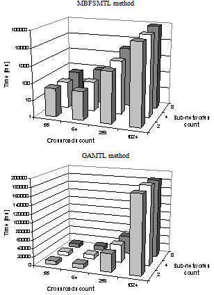Figure 13. Computation time of the MBFSMTL and GAMTL methods

As can be seen in Figure 12 and Table 1, the fastest method for weights assigning is the MaSBWA, which was able to assign weights even for the largest traffic network under 6000 ms. The reason is that the MaSBWA is the only tested method, which utilizes a single simulation run for the weights assigning. The remaining two methods require several simulation runs to be performed to ensure the fidelity of the collected weights. As could be expected, the slowest method is the MiSBWA due to the extreme time requirements of ten simulation runs of the microscopic simulation. Moreover, the simulation memory requirements were at very limits of the 32 bit operating system. So, for even larger traffic networks, the utilization of the MiSBWA method would be impractical. The microscopic simulation was performed directly in the DUTS system instead of the DUTS Editor (see Section 4.3), but the required time was added to the total computation time of the MiSBWA method.

Table 1. Computation Time of the WA Methods Crossroads count Computation time [ms] MaSBWA MeSBWA MiSBWA 55 237 1278 7003 64 268 2709 8653 256 1547 8633 31759 1024 5936 45578 118928

The computation time of the MBFSMTL method depends on the size of the divided traffic network (see Figure 13 (MBFSMTL) and Table 2). It can be also observed that it also depends on the number of resulting sub-networks, especially for larger networks. The highest time was required for marking of traffic lanes of network with 1024 crossroads divided into 8 sub-networks (91231 ms). The lowest time (38 ms) was achieved for the smallest network (55 crossroads) divided into four sub-networks.

Table 2. Computation Time of the MTL Methods Computation time [ms] MTL Crossroads count 2 sub- networks 4 sub- networks 8 sub- networks MBFS 55 47 38 56 64 48 56 113 256 978 1426 3300 1024 52990 60662 91231 GA 55 9069 9187 9250 64 10121 10355 10476 256 42508 42144 42552 1024 180934 185757 184951

Figure 14. MBFSMTL and GAMTL comparison for 8 sub-networks

The computation time of the GAMTL method also depends on the size of the divided traffic network. However, based on the performed tests, it is not influenced by the number of resulting sub-networks (see Figure 13 (GAMTL) and Table 2). The methods is generally slower than the MBFSMTL (see comparison of the methods for 8 resulting sub-networks in Figure 14), but the increase of its computation time with increasing size of the traffic network is slower than that of the MBFSMTL (see Figure 14 and note the logarithmic scale for the MBFSMTL and linear scale for the GAMTL in Figure 13). Also, as it was mentioned above, the MBFSMTL method is dependent on the number of sub-networks.

6.2. Quality of Division of the Methods

Table 3. Simulation Time of the Distributed Road Traffic Simulation Sub-networks count Crossroads count Simulation time [ms] MBFSMTL GAMTL MaSBWA 2 55 12917 10483 64 13837 11099 256 43968 39142 1024 138915 132705 4 55 10359 8506 64 11468 9041 256 32192 26608 1024 92493 88293 8 55 11203 9933 64 13560 11626 256 27073 23407 1024 74280 70541 MeSBWA 2 55 11973 11401 64 13410 11103 256 39700 31459 1024 140516 133255 4 55 10334 8611 64 11448 8975 256 30919 26439 1024 92953 87927 8 55 11301 9663 64 13759 11311 256 26547 22594 1024 73372 71287 MiSBWA 2 55 13519 11264 64 13445 10996 256 41874 37800 1024 138895 131604 4 55 10815 8892 64 11539 8898 256 31013 26062 1024 93422 87987 8 55 11573 10305 64 13888 11073 256 26129 23157 1024 72867 69419

The quality of division of the described methods was tested using the DUTS simulation system on a cluster called Hydra, which is available at DSCE UWB. The cluster consists of ten working nodes. Each node incorporates one CPU Intel Xeon 3.2 GHz, 2 GB of RAM, and 80 GB of hard disk space. The nodes are interconnected with 1 Gbit Ethernet. All nodes are equipped by Debian 5.0.1 operating system.

The tests were prepared as follows. The traffic networks used in previous set of tests (see Section 6.1) were divided by all six combinations of methods for weights assigning and methods for traffic lanes marking. The networks were divided into two, four, and eight sub-networks. These networks were then used for distributed microscopic simulation of the DUTS system performed on the Hydra cluster and the simulation times were measured. The results were averaged from ten simulation runs and are depicted in Table 3.

Generally, the GAMTL method exhibits better quality of division than the MBFSMTL method (see last two columns of Table 3). This means that the distributed simulation of road traffic using the traffic network division by the GAMTL method is faster than using the division by the MBFSMTL method. Hence, it is more convenient to use the GAMTL method, although it is slower than the MBFSMTL method (see Section 6.1).

Regarding the methods for weights assigning, it can be observed that all methods exhibits similar quality of division. This means that the selection of the method for weights assigning has a negligible effect on the resulting performance of the distributed simulation of road traffic. The reason is that the methods assign more-or-less similar weights to the traffic lanes [19], but are variously time-consuming. Hence, it is convenient to utilize the MaSBWA method, since it is the fasted method for weights assigning, which has been tested.

Generally, the results show that, using a convenient division of traffic networks, it is possible to achieve reduction of the simulation time of the distributed simulation (up to 22 % in this case).

7. Future Work

In our future work, we will continue with research of efficient methods for division of traffic network for distributed simulation of road traffic. More specifically, we will focus on several aspects of this issue, which are briefly described in following sections.

7.1. Optimization of Designed Methods

The GAMTL method has several parameters, which influence the result and speed of the method. For example, it is the number of individuals in the generation, number of selected individuals, number of mutation per individual, number of generations, and so on. All of these parameters were set manually based on the preliminary testing of the method. However, this approach does not guarantee the achievement of the optimal results.

For this reason, we plan to utilize a genetic algorithm for optimization of the parameters of the GAMTL method. This approach of “optimizing a genetic algorithm using a genetic algorithm” is likely to be very time-consuming, since it is necessary to perform entire run of the inner genetic algorithm (i.e. the GAMTL method in this case) for calculation of the fitness of one individual of the outer (i.e. optimizing) genetic algorithm. However, since there is a possibility of non-negligible improvement of the GAMTL method, this approach is worth investigating.

The optimization of the MBFSMTL method is also an option. In order to find the best network division, the method attempts to begin the breadth-first search from all crossroads of the network and select the best one. This is a time consuming process, which can be sped up by ignoring of the potentially useless attempts. A heuristic analysis and the knowledge of the traffic networks topology can be helpful with this issue.

7.2. Adaptation for Heterogeneous Environment

The methods for division of traffic network presented in this paper were designed for homogeneous clusters of computers. However, many organizations has a significant amount of computational power distributed among heterogeneous (i.e. with different speeds) interconnected computers (e.g. in computer labs at technical universities). Hence, we will also focus on adaptation of the described methods for the heterogeneous distributed environment.

The methods for weights assigning do not require a modification, since they do not divide the traffic network, but rather only prepare data for the methods for marking of traffic lanes. However, the methods for marking of traffic lanes (i.e. MBFSMTL and GAMTL) would require a slight adaptation for this purpose. It is only necessary for the methods not to divide the traffic network into equally computation-consuming sub-networks, but adapt the size of each sub-network for the speed of the node (computer), on which the simulation of the sub-network will be performed.

For this purpose, it is necessary to know the speeds of all nodes, which will be used for the distributed simulation. It should be noted that the CPU frequency is not viable as a measuring method, since there are other factors influencing the speed of the node. Hence, the speed of each node will be determined by series of the tests. These tests will uncover how large the sub-network should be for each node in order to ensure similar computation time of a simulation time step for all nodes.

For initial testing, these tests will be performed manually. However, remote automated testing of each node is planed for the final version of this approach.

Once the speeds of particular nodes are determined, both MBFSMTL and GAMTL methods can be adapted for heterogeneous division of traffic network by changing of the total weight per sub-network (see Section 5.1) and by changing of the fitness function (see Section 5.2), respectively.

8. Conclusions

In this paper, the performances of several methods for division of road traffic networks were compared. Three methods for weights assigning and two methods for traffic lanes marking were combined into six various approaches for complete division of traffic network into load-balanced sub-networks. All methods were thoroughly tested for their speed and quality of the traffic network division, which they offer.

Considering the speed of the methods and the quality of division, which they offer, the best combination is the MaSBWA and the GAMTL methods together. As it was observed during the testing, the selection of the method for weights assigning has only a negligible effect on the resulting performance of the distributed road traffic simulation. Hence, it is convenient to use the fastest method, which is the MaSBWA. Nevertheless, based on the performed tests, the selection of the method for marking of traffic lanes influences the performance of the distributed road traffic simulation significantly. Hence, it is convenient to use the GAMTL method, which creates better division of traffic network, although it is slower than the MBFSMTL method.

The investigation of the speed of the distributed road traffic simulation using divisions of traffic network by various methods indicates that it is possible to speed up the distributed traffic simulation using a convenient division of the traffic network. Based on the performed tests, the difference of the computation times reached up to 22 %.

In our future work, we will continue with the research of the methods for division of traffic network, as described in previous section.