1. Introduction

Modelling of subsystems of a nuclear power plant is of preponderant importance in order to predict the performance and dynamic analysis of the plant. The ability to predict the plant behaviour at various stages such as steady state, transient state is very essential in order to keep safe operation of the reactor. The complexity of Nuclear Power Plant can be very well seen as large numbers of parameters are used for each sub-system. Hence it is a very intriguing task for the operators to see any unusual events occurring in the reactor due to change in parameter values within a short interval of time. So, at times there may be delay in taking appropriate actions after occurrence of any anomalous events. Several Artificial Intelligence (AI) techniques have been implemented as efficient substitutes to conventional models for semiautonomous operation of the reactor.

Among those, ANN is well suited for the plant dynamic analysis because it has several properties like learning, adaptability, generalizability which outperform the other artificial intelligence techniques. ANN can work efficiently where non-linear functions are used and for evaluating the physical parameters at transient conditions with the help of powerful algorithms like back propagation algorithm[1-6]. The main advantage of ANN is that it can perform interpolation accurately which is of interest of not depending on the process[7]. It is a fast and efficient technique as compared to conventional methods.

Few of earlier works on estimation of parameters and regression analysis using neural network models is cited below. An ANN model is developed for calculating the ferrite content in austenitic stainless steel by[8]. ANN based modelling for pressure drop coefficient for cyclone separators is done by[9]. By physical principles and neural networks, dynamic non linear modelling of power plant is carried out by[10]. A neural research simulator is developed for research reactor dynamics by[11]. To evaluate and predict the deformation behaviour of stainless steel during hot torsion ANN modelling is done by[12]. Nuclear reactor core of VVER has been identified using recurrent neural network by[13]. Neural network based methodology is introduced for cavitation detection in Pressure dropping devices of PFBR by[14]. Neural network is used for safety core parameters prediction in LWRRS by[15] Estimation of low power peaking factor in nuclear fuel is performed using ANN by[16]. PWR system simulation and parameter estimation with neural networks is carried out by[17]. A neural network thermo hydraulic prediction model of advanced nuclear system components is developed by[18]. Classification and prediction of the critical heat flux using fuzzy theory and artificial neural network is performed by[19]. ANN model is developed for dynamic monitoring of simulated operating parameters of high temperature gas cooled engineering reactor by[20]. ANN is modelled for fission gas release in LWR UO2 fuel under RIA conditions by[21].

The objective of this modelling is to evaluate primary and secondary sodium outlet temperatures for given mass flow rate in shell & tube side and respective inlet (primary and secondary) temperatures. The unrealistic temperature prediction for severe unbalanced primary and secondary flow is performed using Nodal Heat Balance (NHB) method,[22]. Later it is modified with the help of Quadratic Upstream Interpolation for Convective Kinetics (QUICK) scheme and from QUICK code the required input data is generated for ANN modelling. The multilayer feed forward network model is observed to be best suited for parameter estimation in IHX. A comparison study of two different algorithms, back propagation and radial basis function algorithm is carried out which showed that RBF showed faster convergence with less number of iterations. The neural network model gave consistent results for training samples.

2. FBTR: A Brief Description

The FBTR is a loop type, sodium cooled reactor which consists of primary sodium circuit, secondary sodium circuit and steam water system. Heat generated in the reactor is transferred from primary sodium circuit to secondary sodium circuit through Intermediate Heat Exchangers. Hence it is very crucial subsystem whose parameter prediction is of utmost importance in a reactor. From secondary sodium circuit, with the help of once through steam generators, heat is transferred to steam water system comprising of turbine generator which in turn produces electricity. In this paper the behaviour of Intermediate Heat Exchanger parameters are examined. The IHX subsystem is explained below.

2.1. Intermediate Heat Exchanger

The Intermediate Heat Exchanger is a vertical, counter flow, shell and tube heat exchanger that transfers heat from active primary sodium to inactive secondary sodium. Primary sodium flows on the shell side and secondary sodium flows on the tube side. It is housed in a fixed vessel with its double envelope. In the reference fast reactor system there are two Intermediate Heat Exchangers in primary circuit, one in each looping[23]. The schematic of IHX is shown in figure 1.

Figure 1. Schematic of sodium-sodium Heat Exchanger of Fast Reactor

When reactor is in operation the control rods are taken out partially so that the neutrons generated can actively participate in the fission reaction which generates heat. The primary sodium will take heat from the radiated core and then will move in upward direction (because of low density property of sodium). Then it will reach up to IHX and enters in radial manner the shell side of IHX at the top. The primary sodium flows vertically downwards and comes out radially at the bottom to the cold pool. The secondary sodium flows upwards inside the tubes. Heat is then transferred from primary sodium to secondary sodium which in turn goes to the steam generator to produce superheated steam. This steam rotates the turbine to generate electricity.

3. QUICK Scheme Simulation

The QUICK scheme is a higher order up winding numerical scheme which takes care of strong convective flow. It uses a three point upstream weighted quadratic interpolation for cell face values. The cell face values of fluxes are always calculated by quadratic interpolation between two upstream nodes and one down stream node. Since the scheme is based on a quadratic function its accuracy in terms of Taylor series truncation error is third order on a uniform mesh,[24]. It is an explicit scheme which uses discretization method which puts values in terms of nodes. The nodes themselves are treated as ordered or discrete values. With the help of QUICK scheme primary and secondary outlet and inlet temperatures have been evaluated for given mass flow rates of sodium-sodium Heat exchanger in shell and tube side.

The outlet temperature of primary and secondary sodium can be estimated using linear interpolation of QUICK scheme and is given in 1a and 1b.

(1a)

(1b)

Here and are primary and secondary sodium outlet temperatures in ℃. The required temperature and flow values of sodium-sodium Heat Exchanger have been generated by running the QUICK code and is used for training the ANN model.

4. Neural Network Methodology

A neural network consists of many simple processing units called neurons which are connected in such a manner that each neuron output further serves as input of generally some more neurons similar to the axon terminals of biological neurons and are connected via synaptic weights with dendrites of other neurons,[25]. The input neurons receive the signals, the working or hidden neurons propagate the signals and the output neurons send the signal output. The architecture of the neural network can be determined by the number of neurons and the layers of neural network. The global dynamics of the neural network can be divided into three modes or phases called as architectural (topological change), computational (state change), and adaptive (configuration change). The architectural dynamics consists of two types of architectures, cyclic (recurrent) where the output layer neuron is feedback to the input layer forming a loop and acyclic (feed forward) where the connections between the layers are disjointedly split into layers where the neurons lead from input to output layer. The computational dynamics tells whether the change of states or updates occur independently (Asynchronous mode) or their updating is centrally controlled (Synchronous mode). It also describes the neural network function (transfer function) is linear or sigmoid or hyperbolic. The adaptive dynamics explains about the initial configuration of the network and how the weights are being updated as a function of time.

The desired neural network is specified by the learning process. Three types of learning processes are there: supervised, reinforcement and unsupervised learning. Supervised learning method always has the desired response, when the inputs are applied and the difference between desired response and actual output becomes the error measure. The error measure is applied next to correct the network parameters. In Reinforcement learning instead of providing the correct output, the teacher determines only the output is right or wrong. Unsupervised learning is always associated with input set of patterns only and the network undergoes change in parameters, discovers patterns, self organizes and determines the features of the network,[26-28]. Some of the application area of neural network includes pattern recognition, prediction and decision making, data compression, regression analysis and control[29].

5. Architecture of Neural Network Model for IHX

For transient condition monitoring of IHX, a multilayer perceptron with feed forward neural network is used. It uses the standard back propagation algorithm as supervised learning method. The multilayer perceptron is designed with three layers, one input layer, one hidden layer and output layer. Variable selection for process modeling of IHX includes identification of the parameters having the most relevant information about the desired output parameters. For IHX the multilayer perceptron has five input nodes in the input layer which include bias, primary inlet temperature, secondary inlet temperature, primary flow and secondary flow. The output layer consists of two output nodes, primary outlet temperature and secondary outlet temperature. The figure 2 shows the architecture of neural network for Heat Exchanger.

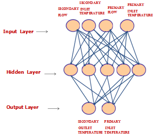Figure 2. ANN architecture for Na-Na Heat Exchanger

6. Training the Neural Network

6.1. Back Propagation Algorithm

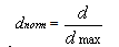
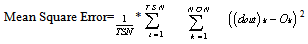
The back propagation algorithm uses the supervised learning which consists of two passes. One is forward pass, where the input values are propagated from input layer to output layer through hidden layer by applying non linear sigmoid function at each layer and finally matching the desired output with the actual output. This generates an error which in squared form is known as mean square error (MSE). Another is backward pass, where the estimated mean square error is back propagated to reduce the weight vectors. This is a non linear optimization process. The main objective of the training process is to adjust weight variables associated the interconnections between layers of ANN so as to make the desired and actual outputs in close agreement with each other.

Since the input data is of wide range, it has to be scaled down between zeros to one which is also known as normalization. The normalization formula used here is

(3)

Where the normalized value of the input and is the input parameter value and is the maximum value of the respective parameters.

The back propagation algorithm is a steepest gradient descent algorithm. The multi layer perceptron is having a nonlinear transfer function known as sigmoid activation function. The activation function has been modified as follows in order to make faster convergence.

(4)

Subsequently fine tuning of the algorithm is required in order to make mean square error as small as possible. To achieve this different number of hidden nodes (NHN) and learning rate parameters (lr) are used and the network is trained so as to fix their values where mean square error is least.

The formula for mean square error is given in equation 5.

(5)

Where is the number of training samples and is the number of outputs and are desired and actual outputs. Careful selection of the learning rate is done because if the learning rate is too small, the convergence is extremely slow and if learning rate is too large, the neural network may not converge at all. One more parameter known as momentum can be used which filters out high-frequency changes in the weight values. By iterating the algorithm the desired weight parameters can be found.

The weight parameters can be calculated using equation 6a and 6b.

(6a)

(6b)

Where, are weight vectors from hidden to output layer and input to hidden layer respectively and W₁, W₂ are the respective weight changes.

6.2. RBF Algorithm

The RBF is a different form of artificial neural network that uses radial basis function as transfer function. RBF is a three layer neural network that uses a linear transfer function for the output units and non linear transfer function for hidden units. The non linear transfer function used here is Gaussian basis function whose output is inversely proportional to the distance from the centre of the neuron and that is stated in equation 7.

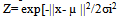(7)

Where Z is the hidden unit output X is the input vector and µ and σ are the centre and width of the basis function. In multilayer perceptron, the network is trained with single global supervised algorithm where as RBF are trained one layer at a time with first layer unsupervised.

The coding has been done in C-language. Out of 77 sets of data the network has been trained with 70 sets of input data generated from the QUICK code. A set of 7 distinct test cases has been chosen within the range of inputs already trained, for testing the network.

7. Results and Discussion

Different trials have been carried out in the training phase to get the optimal values for different number of hidden nodes and learning rates for back propagation algorithm. Figure 3 shows mean square error parameter with respect to the number of iterations for various learning rates and number of hidden nodes. At first the value of learning rate was varied keeping number of hidden nodes constant. Then the number of hidden nodes was varied keeping learning rate constant. The optimal learning rate and number of hidden node for case 1 are NHN=4 and lr =0.01 showing least mean square error= 9.50e-05 for one lakh iterations. The training time taken for 10 lakh iterations is 600 seconds on a typical personal computer system (2.66 GHz Intel Core 2 Duo processor) for 77 training samples.

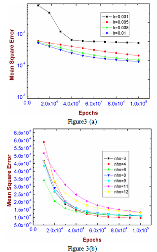Figure 3. Mean square error with respect to number of epochs for (a) various learning rates (b) number of hidden nodes

After fine tuning the network is further trained for 10 lakhs iterations and the results are depicted in figure 4. It shows the graph plotted between the total number of testing sample sets of primary and secondary outlet temperatures for desired and actual outputs. It can easily be seen that the network generate outputs almost matching with the desired outputs and the curves are difficult to distinguish.

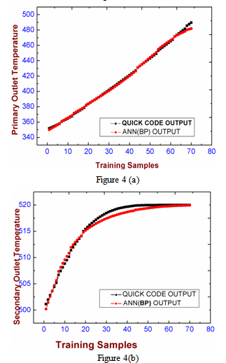Figure 4. Regression analysis for Training sample set using BP algorithm (a) Primary Outlet Temperature (b) Secondary outlet temperature

During testing, the samples within the trained range but not present in the training data set are applied to generate outputs. Fig.5 shows the results obtained during testing with back propagation algorithm. The graph shows that the desired and actual output of primary and secondary outlet temperatures for testing samples overlap with each other and their difference also is very minimal.

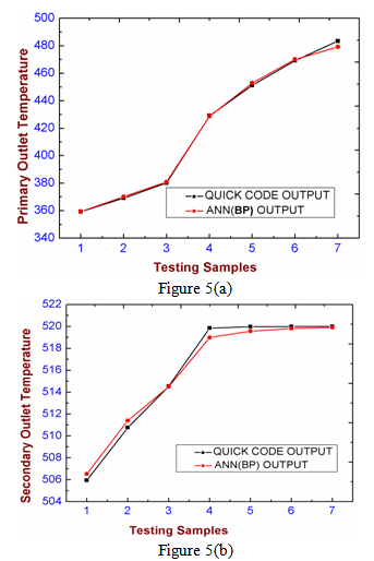Figure 5. Regression analysis for Testing sample set using BP algorithm (a) Primary Outlet Temperature (b) Secondary outlet temperature

In case of RBF neural network, different trials have been conducted with centers varying from 3 to 12 and the optimal numbers of centers are found to be 4. The training results show that it is much faster compared to the standard BP algorithm as the network got converged to 8.92e-06 in 10000 iterations itself. To train the network using RBF it took 160 seconds on a typical personal computer system (2.66 GHz Intel Core 2 Duo processor) with 77 training samples.

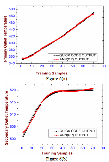Figure 6. Regression analysis for training samples using RBF algorithm (a) desired and actual output for primary outlet temperature and their difference (b) desired output and actual output for secondary outlet temperature and their difference

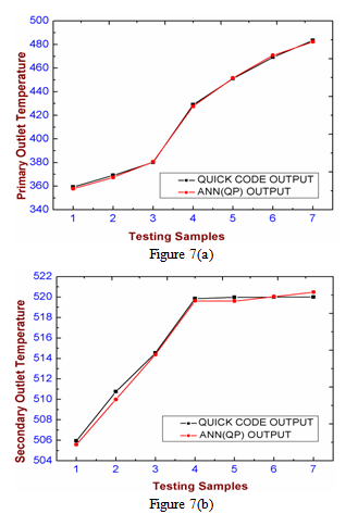Figure 7. Regression analysis for testing samples using RBF algorithm (a) desired and actual output for primary outlet temperature and their difference (b) desired output and actual output for secondary outlet temperature and their difference

Figure 6 and 7 depicts the training and testing results of RBF algorithm. The network is able to generate outputs which are in complete agreement with the desired outputs. This can be represented as ability to generalize. From the results above it can be concluded that compared to the conventional methods used for IHX temperature prediction the standard BP algorithm shows result with less time and compared to standard BP algorithm RBF algorithm converges faster. The standard back propagation has certain drawbacks as it easily gets caught in local minimum instead of reaching the global minimum. This is overcome by RBF algorithm which uses Gaussian function as transfer function.

7.1. Comparison of ANN with Conventional Model

Neural network is preferable as it has faster convergence property and it is less complex than conventional model. Unlike conventional model it does not undergo manual calculations using heuristic equations. Neural network once fine tuned with optimal parameters is able to predict the physical parameters very quickly and accurately.

8. Conclusions

This paper describes the ANN model developed for simulating and studying the steady state and transient conditions of sodium-sodium heat exchanger. The data generated by QUICK Scheme is used for learning phase and further validation. The samples are trained with Multilayer Perceptron using Back Propagation algorithm and is validated with few test samples. From the results it is found that the Neural Network model is able to generalize and produce same outputs which we got from the QUICK code. Another model based on radial basis function neural network is modelled and the results are compared with standard BP algorithm. The training result showed the RBF network is better in terms of fast convergence as compared to standard BP network. These models have fast and accurate prediction capability for both normal and abnormal range of data sets and can be used for plant dynamic analysis. It also helps in studying the behavioural model of the subsystems at steady state and transient states.

ACKNOWLEDGEMENTS

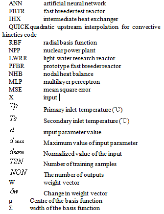
We are immensely thankful to Dr. Sri S.C Chetal, Director, IGCAR, Kalpakkam for his constant support and guidance for this project.

Nomenclature