Deepanwita Das
Department of Information Technology, National Institute of Technology, Durgapur, Burdwan, West Bengal , 713209, India
Correspondence to: Deepanwita Das , Department of Information Technology, National Institute of Technology, Durgapur, Burdwan, West Bengal , 713209, India.
| Email: |  |
Copyright © 2012 Scientific & Academic Publishing. All Rights Reserved.
Abstract
This piece of work studies the partitioning problem on independently operating swarm of autonomous mobile robots and devises algorithms for unbalanced partitioning in a distributed computing environment. The robots considered here are all identical and are very simple and weak. There is no central control over the robots and the robots do not communicate among themselves. Each robot executes the same algorithm based on their local information. This paper frames the algorithms for unbalanced partitioning by sorting the robots based on their ranking and then allocating them in different groups based on their ranks, such that N robots are divided into K unbalanced groups of unequal robots in each group. This paper also presents the performance based analysis of the un-balanced algorithm U_PART over the balanced algorithm and examines their effects via different examples through 50 separate test cases. It also tries to bring out the shortcomings of the proposed U_PART algorithm and proposes another alternative approach towards un-balanced partitioning to overcome the limitation of the U_PART algorithm.
Keywords:
Swarm Robots, Un-balanced Partitioning, Distributed Algorithm
Cite this paper:
Deepanwita Das , "A Distributed Algorithm for Un-balanced Partitioning of a Swarm of Autonomous Mobile Robots and Its Performance Analysis", Advances in Computing, Vol. 2 No. 1, 2012, pp. 17-28. doi: 10.5923/j.ac.20120201.04.
1. Introduction
Swarm robotics is a new approach to the coordination of multi robots which consist of a large number of simple, identical, autonomous and mobile robots over a distributed computing environment[1,2,4]. Such systems mainly consider identical point robots that are oblivious and autonomous, with strong fault tolerance capabilities as a group[5]. These concepts of swarm robotics have various applications such as task allocation[6], military operations, search and rescue victims, lawn mowing and sweeping, space mission, operations like enclosing an invader[8], area exploration and coverage[7] etc. Existing task allocation techniques[6,9, 10] partition the swarm into several groups and dynamically allocate each group of robots to multiple tasks. They may use balanced partitioning techniques[1-3] that partitions n number of robots in k-size balanced groups. But such approach may take large amount of time to complete a job, when groups are allocated multiple tasks with different workloads, as discussed in an example.Consider the problem, where swarm of robots is assigned to paint 50 doors and 50 windows of a building. The area of each window is (3*2)6 square feet and area of each door is(6*3)18 square feet respectively and the swarm contain a total of 10 robots. Say, the whole swarm is partitioned into two groups. Group 1 and group 2 are assigned to colour the windows and doors respectively. As per balanced partitioning each group contains 5 robots. The time required to colour the doors will be greater than to colour the windows by five robots as the total area of the windows is much lesser than the total area of the doors. In this situation, some robots in group 1 will complete its job and remain idle while others in group 2 are still with a larger work load. If the swarm is partitioned in an unbalanced manner of unequal members in each group, then the groups may be allocated task according to the work load, that is, smaller group may be assigned for smaller part of the job (colouring the windows) and the larger group can be assigned for the larger part (colouring the doors). Then no robots will be idle and time required in completing the job will be lesser than that of balanced Partitioning.An algorithm U_Part[4] has been proposed, to partition N number of mobile robots into K number of groups with unequal members in each group. This technique enhances the overall performance of the swarm; as less number of robots will be idle and time required in completing the job will be lesser than that of balanced partitioning. An alternative approach is also presented in the paper as algorithm U_PartII. This paper also studies the performance analysis of the un-balanced algorithm over the existing balanced partitioning techniques presented in[1-3].
2. Related Work
Large amount of research work has been reported on partitioning problem[1-3]. In most of them the robot follows the basic model Wait-Observe-Compute-Move model. Depending on the type of the problem the basic model is modified and used to devise solutions. The algorithms consist of a sequence of computational cycles, which is defined by a sequence of “Look”, “Compute”, and “Move” steps: Look: Whenever a robot becomes active, it observes and marks the positions of all other robots, asynchronously and independently from the other robots, based upon its local coordinate system. Compute: Depending on the observations made in the previous step, the robot calculates its destination point based on its own position and the current locations of the other robots, etc.Move: The robot moves towards the destination point which has been calculated in the compute step.The paper[3] by Asaf Afrima and David Peleg, studies the problem PARTITION(n,k), which partitions n robots in k size balanced groups, and examines the solvability of this problem on various computation model. The algorithm discussed in this paper is PART, Part2, Part_Disperse, Part_Expand, Part_Asym, Part_Sig and Part_Sig2. The paper[1,2] reviews and explores various modification in the basic model developed in[3] and discusses their effects on the solvability of the partitioning problem.David Peleg et. al.[1,2] has considered only balanced partitioning techniques and has stated the basic conditions for partitioning. They are as follows:1. In the FSYNC and SSYNC model, having common axes direction is a necessary and sufficient condition. In ASYNC model, having common axes direction is necessary, and one common axis orientation is sufficient condition for Partition (n, k) to be deterministically solvable for all values of n and k.2. In the ASYNC model, having common axes direction is necessary, and having common axes direction and one common axis orientation is sufficient condition for Partition (n, k) to be deterministically solvable for all values of n and k.3. In the half-compass model, the partitioning problem is solvable in the SSYNC model.4. In the no-compass model, for any timing model, Partition (n, k) is unsolvable for k>1.5. In the axes-only model, for any timing model, Partition (n, k) is unsolvable for some values of n and k.6. In the direction-only model and for the SSYNC timing model, Partition (n, k) is solvable for all values of n and k.So far, the research works on partitioning problem has considered only the balanced approach for partitioning the swarm. In various task allocation techniques, the task load may vary in different groups. In such an environment the balanced partitioning technique will allocate task to groups having equal number of robots in each group. In such a setting, the task load will be more in some groups, whereas in other groups some robots remain unused. As a solution, this paper introduces the unbalanced partitioning techniques.Here, two different algorithms for unbalanced partitioning are presented where a swarm of n robots are partitioned into k unbalanced groups. The first algorithm U_PART presents and unbalanced partitioning technique which creates groups of unequal members of robots. A simulator is being developed to check the time difference in completing distributed workloads, while using balanced and unbalanced group partitioning techniques. Next a comparative performance analysis between balanced and unbalanced techniques[11] has been carried out through the simulator. An algorithm U_Part limits the number of members in each group (except the last group) for all values of N. this limitation has been overcome in the second algorithm U_PartII.
3. Models, Assumptions and Problem Definition
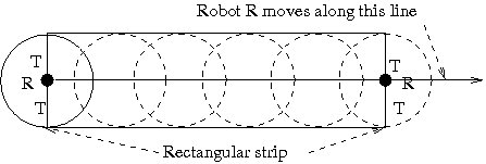 | Figure 1. Sensing zone of radius T |
Before going to describe the algorithm, let us discuss the assumptions and models used, and introduce the terminologies used in this paper. Our problem is to partition n number of robots into k no of size unbalanced groups. These robots are initially deployed within the priori known region. Robots may occupy any position within the region. We assume that no two robots occupy the same position. The robots are assumed to have the following characteristics[7,12]. 1. Identical and Homogeneous - All the robots are identical in all respect, especially, they have the same computational capability. All the robots are assumed to be point robots with unlimited visibility. However, we assume that each of them is having a sensing zone of radius T (T is small). By this we mean that if a robot is required to carry out some job for a particular position (collection of information about that position, or painting that position etc.), instead of actually reaching the position, that can be carried out from a distance of T also as shown in “figure 1”2. Autonomous - There is neither any central authority nor any external control over the robots. They do not even communicate among themselves.3. Mobile - All robots are allowed to move on a plane.4. Computation Model - Here we follow the basic Observe-Compute-Move model. A computational cycle is defined to be a sequence of “observe”, “compute” and “move” steps. Each of the robots executes same instructions in all the computational cycles. Once a robot completes one computational cycle, it starts executing the next one. The actions taken by a robot in compute and move steps, entirely depend on the observations made in observe step. In some situations, an observation might lead a robot not to change its position in move step. In such cases the robot seems to be idle, though it is actually executing all the three steps.5. Oblivious or Memoryless - Robots do not retain any information gathered in the previous computational cycle. In every computational cycle, a robot starts computing from very beginning depending only on the positions of the other robots observed at that computational cycle. The robots can have two states: active and sleep. In Active state, the robots are alive and executing continuously the computational cycles. In Sleep state, robot is not active and doing nothing. This state is like “power off” state. It is assumed that a robot cannot sleep infinitely and it would become active within a finite amount of time. We also assume that change of state of a robot takes place independent of the other robots. The operation considered here is assumed to be an Atomic operation. During the computation process, a robot cannot switch over to the “sleep” state also. The models considered here are as follows:Asynchronous model: Robots operate on independent cycles of variable lengths. They do not share any common clock[7,12].Direction only: Directions of both axes are common to all the robots, but the positive orientation of the axes may be different[7,12]. Here, we assume that x-axes of the robots are parallel to the known common reference line. Therefore, the direction of x-axis is common to all the robots but the robots may have different views of the positive orientation of the axis. However, it is assumed that the direction of the positive y-axis is 90° counter clockwise to the positive direction of the x-axis. Thus, direction of y-axis is also common to all the robots, except possibly the positive orientation. Each robot has its local co-ordinate system. All the robots would assume that they occupy the position (0, 0) with respect to their local co-ordinate system. Further, we assume that these various co-ordinate systems might not share a common scale. “Figure 2” shows the local co-ordinate systems of four robots R1, R2, R3, and R4, and the common reference line XX'. 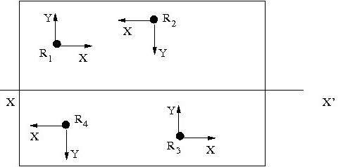 | Figure 2. Local coordinate system of 4 robots |
Lemma 1: The diagonals of a square intersects each other at the center of the square and makes an angle of 90° withLemma 2: The angle traced by a complete circle is equal to 360°.
4. Partitioning Algorithm
The first part of this section describes the proposed algorithm for un-balanced partitioning. The correctness proves of the algorithm are given in the second part.
4.1. Algorithm for Unbalanced Partitioning
This research work proposed an algorithm to partition N number of robots into K number of unbalanced groups. Further, we assume that all N robots are enclosed within a known obstacle free square region The robots need to be partitioned into K (Gr1, Gr2, Gr3 ,…., Grk )number of size-unbalanced groups. As the groups will not be balanced in size, so the total number of robots in each group always differs with the number of members in all other groups.To create such unbalanced groups, each group will contain number of members equal to the group number except the last group which may or may not contain same number of robots equal to the group number depending on the value of N. As the group number and the number of members in a group are same, so now onwards value of group number is considered as the number of members in that group. Each robot contains a flag (FLAG) which is set with the value of the particular group number to which the robot is assigned. As soon as a robot R becomes alive it performs the following computational cycle “observe-compute-move”. As long as a robot is in alive state, after completing one such computational cycle, it would again start another cycle and continue in this way until it completes its assigned job. Each robot in the swarm executes same algorithm U_PART when active.In the look state a robot gathers information of its neighbour. Then it computes its rank, group number and goal point. The rank is calculated with the help of the observed information. Using the rank of the robot its group number is calculated. The robot needs to move towards the respective goal points to form the partition. The number of goal points is same as the number of groups formed. So the goal point of robot R is calculated in the compute step. It moves to the goal point in the move step.Algorithm U_PART (Executed by Robot R)Look:According to the local co-ordinate system, a robot R first observes the position of all other robots. Let the co-ordinates be (a1, b1), (a2, b2), …. (an-1, bn-1), whereas, its own co-ordinate would be (0,0). It is to be noted here that some of these ai, bi values might be negative also.Compute:Step 1: According to the values of y-co-ordinates, the robot R will order all the robots (including itself) so that the robot having the largest value of y coordinate will have the highest rank, that is, N. Without loss of generality, we assume that the co-ordinates of N robots, after sorting are (x1, y1), (x2, y2), (xN, yN), so that (y1<=y2<=y3<=... yN). The robot having the co-ordinate (xi, yi) would have the rank i and the robot will be mentioned as Ri, 1<=i<=N. In case of a tie, the values of x-coordinate of the robots are considered. The robot having lower x-coordinate would have the lower rank.In case of tie in the value of y-coordinate, means two robots are in a same location which is not possible practically. In this way, the robot R would determine its own rank. Let the rank of R be p. From now onwards R and Rp will be used interchangeably. Step 2: The value of “K” that is; the total number of groups formed should be K<=ceiling (N/2) and must be selected in such a manner that no two groups contain equal number of robots. Step 3: Once a robot gets its rank it checks whether it is having the lowest or highest rank among all other robots. The lowest ranked robot always belongs to the first group and the highest ranked robots belong to the last group.Step 4: If the robot is having rank “p” which is neither lowest nor highest, it checks whether p<=1+Gr1, if true it then sets the FLAG=2. If false it again checks p<=1+Gr2+Gr3, if true it sets FLAG=3. For each false outcome the rank is checked against the previous cumulative sum added to the next group number. This checking continues till p<= (K(K-1))/2. If true, then FLAG=(K-1). If false then robot will be assigned to the Kth group.Step 5: The robot R computes the group number to which it is allocated. It then needs to compute the goal point towards which it must move to form the partition. The robot R calculates the center of the square field which is the intersection of the diagonals. Now the robot R first checks its group number. If it belongs to group 1 then, it computes its goal point by calculating an angle Θ (theta) where Θ=45°, from the center point in anti-clockwise direction along the line XX' and marks its goal point at a fixed distance “d” from the center, considering d<=a/4 where “a” is the dimension of the side of the square. If the robot R belongs to group 2, it then computes its goal point at an angle 2Θ at a distance “d” from the center. In this way the value of Θ increases with the group number till Θ reaches 360° or 8 Θ.If the group number exceeds 8(GrK>8) then the robot R computes the goal point at an angle Θ=45° at a distance 2d from the center. The angle Θ increases in the same order as before and continues till it completes 360° or 8 Θ for group number 16 in the second round. In this manner the goal point is calculated over the square field based on the group numbers to which a robot belongs. After completing each round of 360° the distance increases by “d”' and the angle begins from Θ every time.To maintain the relative ranking throughout the process, the robot R may need to take a halt before reaching its final destination. In this compute step, the robot R should verify this situation and if required, it would recalculate the position of the halt. We call this as the secondary destination.The “compute” step terminates as soon as the robot computes its destination, final or secondary. The “Figure 3” below shows the different goal points of the groups.Move:After identifying the goal point, the Robot R starts moving towards the goal point. On the way towards their destination, robots would maintain their relative ranking. It means, while moving, robots should not cross vertically any other robot even if their routes do not intersect each other. In other words, to reach the destination, if a robot is going to gain a vertical height higher (lower) than a robot of higher (lower) rank (that is, it is crossing another robot which would affect the relative ranking), it would stop at an € (pre-defined small quantity) distance from that height and would wait for that other robot to move on. In this situation, the robot R may need to take a halt before reaching its final destination and if required it will recalculate the position of next halt. This halts are known as secondary destination. 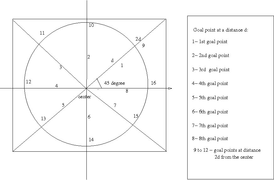 | Figure 3. Different goal points for different robots |
A robot would always move in vertical direction first, after acquiring the vertical height of the final destination, the robot would then move into horizontal direction to reach the final destination. Thus, to reach the secondary destination, a robot moves only in vertical direction. Depending on whether a robot reaches its final or secondary destination, the following two courses of actions would be taken by the robot:(i) As soon as, a robot reaches the secondary destination, this “move” state terminates. That is, the computational cycle will be terminated and the robot will again start a new computational cycle with “observe” state.(ii) Once the robot reaches its final destination that means the job is completed successfully, without any interruption. At the end, it would generate a signal that its job is done. At any point of time, if the robot R finds another robot R’ at the same vertical height (which might occur at the starting time, if initially they are at the same height), then depending on the rank of R’ and that of itself, R decides its next course of action as follows:Case A: The rank of R is greater than that of R’ and the destination of R is in the positive direction, w.r.t. its local co-ordinate system.Case B: The rank of R is less than that of R’ and the destination of R is in the negative direction, w.r.t. its local co-ordinate system.For both the cases, R would break the tie and would move first towards its destination point.Case C: The rank of R is greater than that of R’ and the destination of R is in the negative direction, w.r.t. its local co-ordinate system.Case D: The rank of R is less than that of R’ and the destination of R is in the positive direction, w.r.t. its local co-ordinate system.For both the cases R will wait for R’ to move first towards its destination point.
4.2. Correctness Proofs
4.2.1. Observation 1: The Overall Process Starts at a Finite Amount of Time
Proof: As mentioned before, the robots can have two states: active and sleep. In Active state, the robots are alive and executing continuously the computational cycles. In Sleep state, robot is not active and doing nothing. This state is like power off state. It is assumed that a robot cannot sleep infinitely and it would become active within a finite amount of time. We also assume that change of state of a robot takes place independent of the other robots. Thus whenever a robot becomes active it executes the algorithm and it is also assumed that the other robots will also become active after a finite time and will execute the same algorithm independently. Hence it is guaranteed that overall process starts at a finite time.Only in case of a tie, if initially the robots are at the same height, there will be inter-dependency among these robots. If a particular robot do not move first all other have to wait for it and so on. The robot having the highest rank and the lowest rank usually does not have any restriction on their movement and thus as soon as they become live, the process starts. An extreme situation is considered when all the robots are at the same height.The situation can be sub-divided into following two cases:Case 1: All the robots are at the same height and they are along a boundary of the region. In this case, if a robot identify itself (according to its local co-ordinate system) (1) at the lower boundary of the region and having the highest rank, or (2) at the upper boundary of the region and having the lowest rank.In both of the cases the robots will not have any restriction on its movement and it would break the initial barrier. These robots are called tie-breaking robots. If the robots are on the upper boundary, the left-most one and if they are on the lower boundary, the right-most one will be the tie-breaking robot.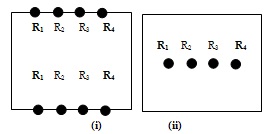 | Figure 4. R1 and R4 are the tie-breaking robots in two cases |
Case 2: All the robots are at a same height from the common reference line but they are not along any boundary of the region. In this case both the robots having lowest rank and highest rank will not have any restriction on their movement and they would break the initial barrier. “Figure 4”, below shows both the cases where the tie-breaking robots either having highest or lowest rank. Once a robot break the initial barrier, all other robots start moving in turn. Thus within finite time the process would start.
4.2.2. Observation 2
Throughout the process, relative ranking of the robots computed by several robots are same up to a reversal of order. In other words, if the robots R1 and R2 compute the rank of a robot R as i and j respectively, then either i=j or i= N-j and this would remain same throughout the algorithm.Proof: If the orientations of the local axes of R1 and R2 are identical then the ranking of the robots would be same. Otherwise, if the orientations are reverse, then the relative ranking would be same but in reverse order. Thus i=N-j. “Figure 5” shows the positions of five robots and their ranks with respect to robots A and E. Robots A and E are having opposite orientations. The ranks of the robots w.r.t A are just the reverse of the ranks w.r.t E.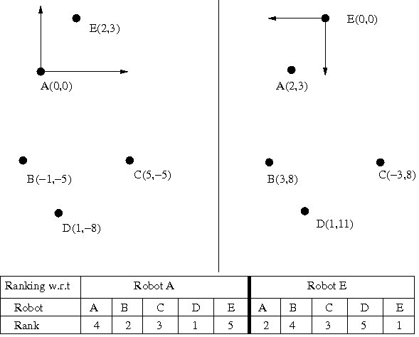 | Figure 5. Relative ranks w.r.t robot A and E are same up to a reversal of order |
A robot computes the ranks of all other robots w.r.t. their vertical distances from its local x-axis. So the relative ranking of the robots would remain same throughout the algorithm as the vertical movement of the robots is so restricted that none of the robots would vertically cross any other robot.If two robots are starting from the same vertical height, their relative ranking will be determined by their x- coordinates.In case of such a tie, the robots start moving towards their destination following the rule given in “move” step, which retains their relative ranking.Once a robot starts moving, this tie will be broken and this situation will never occur again.
4.2.3. Observation 3: The Group Number Allocated to the Robots Remains Same Throughout the Process
Proof: Robot R is allotted its group number according to its rank. Thus group 1 contains 1 robot, group 2 contains 2 robots of rank 2 and 3, and in this way (K-1) group contains “K-1” number of robots. Thus remaining robots (N-(1+2+3+….+K-1))=N-(K(K-1))/2 is contained in the Kth group and flag assigned is GrK. As the relative ranking is preserved and does not change throughout the algorithm henceforth the group number is preserved.Example: Let us consider 6 robots, with relative ranking 1, 2, and 3, 4, 5, 6. Now the group numbers allocated will be as follows: Robot with rank 1 is assigned group 1, robots with ranks 2, 3 is assigned group 2 and robots with ranks 4, 5, 6 are assigned group3. Thus if the relative ranking remains unchanged throughout the process then the group numbers allocated will certainly remain fixed throughout the process.
4.2.4. Observation 4: Θ is Always Equal to 45° and 8Θ Completes a Circle Around the Center Point
Proof: The robot R calculates the center of the square field which is the intersection of the diagonals. Now the robot R first checks its group number. If it belongs to group 1 then, it computes its goal point by calculating an angle Θ (Θ=45°) from the center point in anti-clockwise direction and marks its goal point at a fixed distance d from the center, considering d<=a/4 where “a”' is the dimension of the side of the square.Since the field is square in shape, by Lemma 1 above the angle made at the center by the diagonals are 90°. The center line parallel to x-axis passing through the center of the square field makes an angle of 45° with the diagonals. Thus Θ is taken as 45°. Now the goal point is calculated at an angle Θ at a distance d from the center if robot R belongs to group 1, considering d<=a/4 where “a” is the dimension of the side of the square. If robot R belongs to group 2 the goal point is calculated at an angle 2Θ from the center at a distance d from the center. In this way the angle increases linearly as the group number increases till 8Θ. If the group number crosses 8, then the next angle again starts from Θ and the goal point is calculated at a distance 2d from the center and continues till it reaches 8Θ. After every round of 8Θ the next goal point is calculated at an angle Θ and the distance from the center is incremented by d. By Lemma 2 8x45°=360° completes one circle around the center point. Therefore the group numbers belonging to 8, 16, 32, 64 which consist of a GP series make an angle of 8Θ every time on completing 360° and the next group numbers belonging to 9, 17, 33, 65 starts calculating the goal point from the center of the field along the line passing through the center at an angle of Θ.
4.2.5. Observation 5: The Partitioning Algorithm Results an Unbalanced Groups of Robots
Proof: In the algorithm U_PART above the robots are grouped according to their ranks. Thus group 1 contains 1 robot, group 2 contains 2 robots of ranks 2 and 3, and in this way (K-1) group contains K-1 number of robots. Thus remaining robots (N-(1+2+3+….+K-1))=N-(K(K-1))/2 is contained in the Kth group and flag assigned is GrK. Let us consider two cases as follows:Case 1: Let 10 robots be present in the field. Then by the algorithm U_PART, the 10 robots ranked from 1 to 10, by unbalanced partitioning robot R1 is assigned group Gr1, R2 and R3 are assigned Gr2, R4, R5, R6 is assigned Gr3 and robots R7, R8, R9 and R10 is assigned Gr4. The algorithm works correctly if the formula (N-(1+2+3+...K-1))=N-(K(K-1))/2 gives the same outcome. Verifying the formula: (n-(1+2+3+...k-1))=n-(k(k-1)). For N=10 and selecting K=4, since K<=ceiling (N/2)=(10/2)=5, therefore N-(K(K-1))/2=10-(4(4-1))/2=10-(4x3)/2=10-6=4. Therefore there must be 4 robots present in the Kth group. As the outcome matches with the result obtained from the formula, the algorithm U_PART works correctly.Case 2: Now, considering for N=11 robots, K=4, since K<=ceiling (N/2). Now, N-(K(K-1))/2=11-(4x3)/2=11-6=5. Therefore there are 5 robots present in the last group or group 4 in this case. Thus each group will contain number of members equal to the group number except the last group which may or may not contain same number of robots equal to the group number depending on the value of N, therefore Gr1 will contain 1 robot, Gr2 will contain 2 robots, ….,GrK will contain [(2N-K(K-1))/2] ,where unbalanced partition is guaranteed.Henceforth it must also be kept in mind that the group number is so selected that no two groups have equal number of robots. Therefore unbalance partitioning is guaranteed.
4.2.6. Observation 6: The Movement of the Robots is Collision Free
Proof: Throughout the algorithm, two robots can never be at the same vertical height at the same time, except during the starting time, when two robots can be at the same vertical height. If initially the robots are at the same height, the tie is broken by the rules given in Move step. Once the tie is broken, they will never be at the same height again, during their vertical movement.After computing the destination, each robot would first move vertically to reach the height of the final destination. Once they reach that height, they start moving horizontally. Thus, if the destinations of the two robots are at different heights, the question of collision during their horizontal movements does not arise at all.
4.2.7. Observation 7: The Four Rules Stated in the Move Step are Valid
Proof: If at the initial stage, two robots are at the same height(but in two different positions), the robot having the higher rank would start moving first, if their destinations are in the negative direction, then the robot having the lower rank would start moving first. If their destinations are in opposite direction, then there wouldn't be any restriction in the vertical movement. Consider “figure 6” below where both R1 and R2 have the same orientations. The destinations of robots R1 and R2 are d1 and d2 respectively. According to both the robots the rank of R1 is less than the rank of robot R2. In the “figure 6(a)” both of their destinations are in the positive direction, then as per the rule, the higher ranked robot R2 will move first. In “figure 6(b)” both of their destinations are in the negative direction. As per rule, the lower ranked robot R1 will move first. 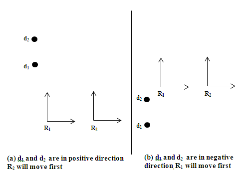 | Figure 6. R1 and R2 are having same orientation |
Consider “figure 7” where both R1 and R2 having opposite orientation. According to the local coordinate system of R1 and R2, both will rank itself as lower. Due to opposite orientations, if the destinations are in positive direction according to R1 then it is in negative direction according to R2 and vice versa. 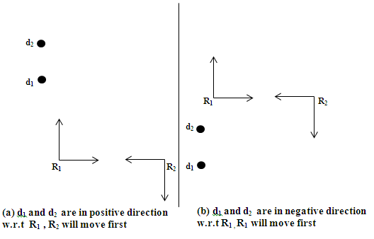 | Figure 7. R1 and R2 are having opposite orientation |
In “figure 7(a)” both the destinations are in the positive direction w.r.t R1. So, according to R1, the higher ranked robot R2 will move first. But according to R2 the destinations are in negative direction, so as per rule the lower ranked robot R2 will move first. This shows that the same decision will be taken by R1 and R2. Similarly, in “figure 7(b)”, both the destinations are in negative direction w.r.t R1. So, according to R1, the lower ranked robot R1 will move first. But according to R2 the destinations are in positive direction, so as per rule higher ranked robot will move first which is R1 according to the local coordinate system of R2. So, in both the cases same robot will move, and the tie will be broken without any conflict.
4.2.8. Result: The Partitioning Algorithm U_PART Will Be Completed Within a Finite Amount of Time
Proof: Combining all the above observations, and the fact that a robot cannot sleep for infinite amount of time and considering the operation to be atomic, we conclude that the overall process completes successfully within finite amount of time.
5. Simulation and Performance Analysis of Algorithm U_PART
5.1. Simulation
In this section, the two partitioning techniques has been compared and analysed. An example of an academic building has been considered. The building is assumed to have a number of lecture rooms. Different number of chairs is placed in each room. A swarm of robots have been allocated to colour all the chairs placed in different rooms of the building. Colouring all the chairs in one room is considered as one task. Both the algorithms suggest partitioning the robot swarm into number of groups so that each group can complete at most one task. Assuming that numbers of groups are equal to the number of task to be done. A simulator has been developed to evaluate and compare the overall performance of un-balanced algorithm over the balanced algorithm. 50 test cases have been analysed using the simulator to study the performance of the un-balanced algorithm over balanced algorithm. The simulator calculates the total time required to complete the whole job (painting all the chairs in all the rooms of the building) by the swarm by applying the balanced algorithm as well as the un-balanced algorithm. Based on the comparison of time required to complete the job the simulator suggests the technique to be used for a particular task to be done in minimum time.
5.2. System Requirements of the Simulator
5.2.1. Software:
Turbo C++ version 4.5 compiler, Matlab 7, Windows XP Professional (SP2)
5.2.2. Hardware
Processor: Pentium IV 1.4 GHz minimum, Disk Space: 2 GB, RAM: 1024 MB, DVD ROM drive, High resolution monitor (XGA recommended), Keyboard and Mouse.
5.3. Performance Analysis
The simulator studied 50 test cases to evaluate the performance of the unbalanced algorithm over the balanced algorithm. A swarm is allocated to colour all the chairs situated in different rooms inside the building. Colouring all the chairs in one room is considered as one task. It is assumed that one robot can paint a single chair within 5 minutes. The task is carried out concurrently by individual robot.N = Number of robots in the swarm.K = Number of groups formed.Ci = Number of chairs present in the ith room.Tib = Time taken to colour all the chairs in the ith room, in minutes by balanced partitioning.Tiub = Time taken to colour all the chairs in the ith room, in minutes by un-balanced partitioning.TOB = Maximum time taken to complete colouring all the chairs present inside the building via balanced partitioning.TOUB = Maximum time taken to complete colouring all the chairs present inside the building via un-balanced partitioning.The tables in Appendix A (table no A.1& A.2) shows the results obtained from 50 test cases. Out of 50 test cases mentioned above, 3 random cases have been plotted to bring out the comparison between balanced and un-balanced techniques.Problem 1: The building has two rooms, having 10 and 160 chairs respectively. The swarm is partitioned into two groups (one group per task) using balanced as well as unbalanced partitioning. Then the total time required to complete the task is compared and analysed for both partitioning techniques.Problem 2: The building has three rooms, having 2, 50 and 300 chairs respectively. The swarm is partitioned into three groups using balanced as well as unbalanced partitioning. Then the total time required to complete the task is compared and analysed for both partitioning techniques.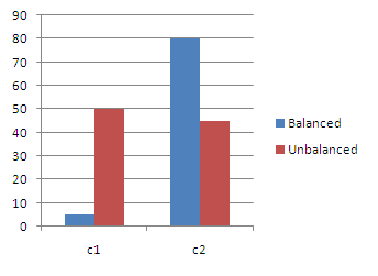 | Figure 8. Represents problem 1 |
Problem 3: The building has four rooms, having 4, 40, 80 and 200 chairs respectively. The swarm is partitioned into four groups using balanced as well as unbalanced partitioning. Then the total time required to complete the task is compared and analysed for both partitioning techniques. “Figure 8”, “figure 9” and “figure 10” plots the number of chairs to be collared along the x-axis and the time in minutes along the y-axis.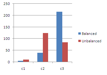 | Figure 9. Represents problem 2 |
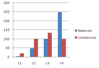 | Figure 10. Represents problem 3 |
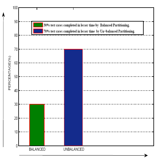 | Figure 11. Statistical representation |
Result: Out of the 50 test cases analysed, 70 percent of the cases prefer un-balanced partitioning and 30 percent of the cases support balanced partitioning with respect to time. “Figure 11”, shows the statistical representation of cases for both balanced and un-balanced partitioning techniques respectively.The following conclusions can be made from the experiments carried out:(i) Un-balanced partitioning is advantageous for uneven task distribution where the task difference between the groups is huge. In such situations, the time taken to complete the total task is more in comparison to un-balanced partitioning.(ii) Algorithm U_PART is useful when the task distribution between the groups increases in ascending order with huge difference between each group.(iii) With respect to time, un-balanced partitioning gains advantage over balanced partitioning, as the value of K increases and when the last group contains huge task load compared to other groups.(iv) Balanced partitioning is not possible for any prime value of N and also for all N, K pairs where K does not divides N. As there are no such restrictions for un-balanced partitioning, hence U_PART algorithm partitions N for a wide range of values K.Thus it can be concluded that for certain applications, where un-even task distribution is required; un-balanced partitioning is more advantageous compared to balanced partitioning.
6. An Alternative Approach to Unbalanced Partitioning
6.1. Limitation of U_PART Algorithm
Although, algorithm U_PART works well for a large value of N, K pairs but it limits the members in each group to its group number except the last group, for all values of N.This limitation has been overcome in the next section, where an alternative approach has been taken into consideration towards un-balanced partitioning and an un-balanced algorithm U_PART II has been proposed.
6.2. Algorithm: Unbalanced Partitioning II
This section proposes another algorithm to partition N number of robots into K number of unbalanced groups. All assumptions are same as the first algorithm. On being active each robot uses an array m[50] which stores the number of members present in each group and a variable s which stores the sum of the members in each group, except the last group. Algorithm U_PARTII (Executed by Robot R)Look: The Look step remains same as in algorithm U_PART.Compute:Step 1: This step remains same as in algorithm U_PART.Step 2: Next, robot R checks whether (K==2), if true then there are only two groups. Member in Gr1 is m1=(N/2) and Gr2 is m2=(N-m1), where m1 and m2 (which stores only integer values and the fractional part if any is truncated), represents the number of members in Gr1 and Gr2 respectively. Next, it is checked if(m1==m2); if true then set m1=m1-1 and set (m2=m2+1). Otherwise go to step 3.Step 3: If (K!=2) then robot R initializes i=0; and for each value of i, it sets m[i]=(N/K-i) (m[i] stores only integer values and the fractional part s are truncated) and increments the value (i=i+1) till (ith group, Gri+1.Step 4: R initializes s=0; and stores the sum of all m[i] values in variable s for all values of i; it updates s=s+m[i] for every value of i and checks whether s exceeds N; i.e.; (sth group, GrK. Otherwise go to step 5.Step 5: If (s>=N) is true then R decides that only (K-1) groups are possible and updates s=s-m[i] and assigns ml=N-s; where ml represents the number of members in the (K-1)th group, GrK-1.Step 6: After robot R calculates the number of members in each group it then decides its own group number. R first initializes i=0; If the robot is having rank “p”, it checks whether p<=m[i], if true it then sets the FLAG=i+1. If false it increments the value of I by 1 and checks if p<=m[i]+m[i+1]. If true it sets FLAG=i+2; for each false outcome the value of i is incremented by 1 and the rank p is checked against the previous cumulative sum added to the next group members. The checking continues till i<(K-1), where K groups are possible (otherwise it continues till i<(K-2)). If false R is allocated to Kth group and sets its FLAG=K. Otherwise it belongs to GrK-1; FLAG=K-1 for (K-1) groups.Step 7: This step remains same as in algorithm U_PART step 5.Move: The move step remains same as in algorithm U_PART.
6.3. Correctness Proofs for U_Part II
6.3.1. Observations
All the observations mentioned in algorithm U_PART remains same and are all valid for algorithm U_PARTII. The algorithm U_PARTII guarantees un-balanced partitioning. Let us consider the flowing cases below:Case 1: Let N=10, i.e.; robots present in the field and K=2. Then by the algorithm U_PARTII, the 10 robots ranked from 1 to 10. As K=2, by U_PARTII; m1=(N/2)=10/2=5; m2=N-5=5; now since(m1==m2) we set m1=m1-1 and m2=m2+1; hence m1=5-1=4; m2=5+1=6. Robot R1, R2, R3, R4 is assigned group Gr1 as rank p<=m1 and R5, R6, R7, R8, R9, R10 belongs to Gr2 by algorithm U_PARTII.Case 2: Let N=25 and K=3. Then by algorithm U_PARTII, the 25 robots are ranked from 1 to 25. As here K>2, by U_PARTII; i=0, s=0; as m[i]=(N/K-i); m[1]=25/(3-0)=8 (taking only the truncated value); m[2]=25/(3-1)=25/2=12 and s=s+m[0]+m[1]=20; as (20i+1= Gr1 contains 8 members; similarly Gr2 contains 12 members and Gr3 contains 5 members. Robot R1, R2, R3, …., R8 is assigned group Gr1 as rank p<=m[0] and R9, R10, R11,…., R20 belongs to Gr2 since p<=m[0]+m[1]=12+8=20 and finally R21, R22, R23,…., R25 belongs to Gr3.
6.3.2. Result: The partitioning algorithm U_PARTII will be completed within a finite amount of time
6.4. Limitation of Algorithm U_PARTII
The U_PARTII algorithm overcomes the shortcomings of U_PART algorithm by allocating members to groups which are not fixed for all values of N. But it does not guarantee partitions for a wide range of values of K. Let us take up two examples to bring out the limitation:Case 1: For N=10 and K=2; Gr1 and Gr2 contains m1=4 and m2=6 members each.Case 2: For N=25 and K=5; Members in group 1 = 5; Members in group 2 = 6; Members in group 3 = 8; Members in group 4 = 6. For this value of n=25, only 4 groups are possible.Thus U_PARTII algorithm guarantees un-balanced partitioning but does not guarantees partitioning for all values of K. We may try to overcome this limitation in our future work.
7. Conclusions
The development in the field of swarm robotics is reaching a point where various new applications are emerging. Here we have dealt with the partitioning problem where swarm of autonomous robots are balanced partitioned into equal groups of robots and have proposed our own partitioning techniques for un-balanced partitioning.In case of un-balanced task allocation the balanced partitioning becomes disadvantageous from the time consuming point of view, thus in such an environment unbalanced partitioning has been introduced, where a swarm of robots are partitioned into K unbalanced groups.The algorithm U_PART partitions a swarm of robots in an unbalanced way over a square field. If the area considered is rectangle or polygonal in shape, then the partitioning can be done in similar manner. To bring out the benefits of the algorithm U_PART, a simulator has been created, where 50 experiments have been carried out. Based on the results obtained from the 50 test cases, it can be concluded that U_PART algorithm performs better than the balanced algorithm for certain applications which uses uneven task distribution techniques.As U_PART algorithm allocates fixed number of robots for each group except the last group; for all values of $N$, we have proposed another alternative approach towards un-balanced partitioning to overcome this limitation via algorithm U_PARTII. Although the algorithm U_PARTII overcomes the limitation of algorithm U_PART but does not guarantees partitioning for all values of K.Henceforth, it may be concluded that the two alternative approaches for unbalanced partitioning certainly have their own limitations, but at the same time are useful for particular purposes and can be used alternatively as the situation demands.
8. Future Work
This piece of research work proposes two un-balanced partitioning approach on a swarm of autonomous mobile robots. Here two algorithms U_PART and U_PARTII have been proposed which overcomes the shortcomings of the balanced algorithm, where N robots have been partitioned into K unbalanced groups. .Here a square field has been considered over which the robots are placed for partitioning; the algorithm can also be performed over a rectangle or polygonal field of known or unknown dimension, in similar manner. Both the algorithms have certain limitations which may be taken up as future scopes of study: (i) Overcoming the limitation on fixed number of members in a group in the algorithm U_PART. (ii) Overcoming the limitation on partitioning for wide range of K values in the algorithm U_PARTII. (iii) Moreover, an obstacle-less field has been considered for both the techniques. In practical cases there may be situations where the robots are placed in a field where obstacles are present. It may be aimed at devising an algorithm in future for unbalanced partitioning which will work in such environment also. (iv) The robots considered here has unlimited visibility capabilities. In future research work, the algorithm may be extended to support limited visibility of the robots as well.
ACKNOWLEDGEMENTS
We would like to acknowledge the generous support of the Department of Information Technology of National Institute of Technology, Durgapur.
Appendix a
| Table A.1. Result of Simulation: 35 test cases supporting unbalanced partitioning |
| | Test Cases | Ci =Task in each group | Tib | Tiub | TOB | TOUB | | Case 1: N=10, K=2 | 10 | 10 | 50 | 110 | 65 | | 110 | 110 | 65 | | Case 2: N=10, K=2 | 23 | 25 | 115 | 325 | 180 | | 322 | 325 | 180 | | Case 3: N=12, K=3 | 2 | 5 | 10 | 125 | 60 | | 20 | 25 | 50 | | 100 | 125 | 60 | | Case 4: N=12, K=4 | 2 | 5 | 10 | 170 | 85 | | 20 | 35 | 50 | | 50 | 85 | 85 | | 100 | 170 | 85 | | Case 5: N=15, K=3 | 3 | 5 | 15 | 90 | 75 | | 30 | 30 | 75 | | 90 | 90 | 40 | | Case 6: N=16, K=4 | 4 | 5 | 20 | 250 | 135 | | 40 | 50 | 10 | | 80 | 100 | 135 | | 200 | 250 | 100 | | Case 7: N=20, K=5 | 14 | 20 | 70 | 135 | 95 | | 35 | 45 | 90 | | 55 | 70 | 95 | | 75 | 95 | 95 | | 105 | 135 | 55 | | Case 8: N=21, K=3 | 2 | 5 | 10 | 215 | 125 | | 50 | 40 | 125 | | 300 | 215 | 85 | | Case 9: N=25, K=5 | 1 | 5 | 5 | 55 | 35 | | 5 | 5 | 15 | | 15 | 15 | 25 | | 25 | 25 | 35 | | 55 | 55 | 20 | | Case 10: N=30, K=5 | 20 | 20 | 100 | 170 | 125 | | 40 | 35 | 100 | | 60 | 50 | 100 | | 100 | 85 | 125 | | 200 | 170 | 50 | | Case 11: N=20, K=2 | 10 | 5 | 50 | 80 | 50 | | 160 | 80 | 45 | | Case 12: N=12, K=3 | 2 | 5 | 10 | 375 | 170 | | 28 | 35 | 70 | | 300 | 375 | 170 | | Case 13: N=18, K=3 | 3 | 5 | 15 | 170 | 70 | | 10 | 10 | 25 | | 200 | 170 | 70 | | Case 14: N=27, K=3 | 2 | 5 | 10 | 60 | 25 | | 8 | 5 | 20 | | 100 | 60 | 25 | | Case 15: N=27, K=3 | 5 | 5 | 25 | 55 | 25 | | 10 | 10 | 25 | | 95 | 55 | 20 | | Case 16: N=27, K=3 | 5 | 5 | 25 | 170 | 65 | | 25 | 15 | 65 | | 300 | 170 | 65 | | Case 17: N=50, K=5 | 2 | 5 | 10 | 45 | 20 | | 5 | 5 | 15 | | 10 | 5 | 20 | | 11 | 10 | 15 | | 90 | 45 | 15 | | Case 18: N=111, K=3 | 1 | 5 | 5 | 10 | 5 | | 2 | 5 | 5 | | 50 | 10 | 5 | | Case 19: N=9, K=3 | 2 | 5 | 10 | 15 | 10 | | 3 | 5 | 10 | | 9 | 15 | 10 | | Case 20: N=6, K=3 | 3 | 10 | 15 | 20 | 15 | | 5 | 15 | 15 | | 7 | 20 | 15 | | Case 21: N=10, K=2 | 2 | 5 | 10 | 170 | 95 | | 170 | 170 | 95 | | Case 22: N=15, K=5 | 2 | 5 | 10 | 85 | 50 | | 5 | 10 | 15 | | 10 | 20 | 20 | | 30 | 50 | 40 | | 50 | 85 | 50 | | Case 23: N=90, K=10 | 9 | 5 | 45 | 55 | 50 | | 10 | 10 | 25 | | 22 | 15 | 40 | | 33 | 20 | 45 | | 44 | 25 | 45 | | 55 | 35 | 50 | | 66 | 40 | 50 | | 77 | 45 | 50 | | 88 | 50 | 50 | | 99 | 55 | 15 | | Case 24: N=80, K=10 | 8 | 5 | 40 | 60 | 45 | | 10 | 10 | 25 | | 20 | 15 | 35 | | 30 | 20 | 40 | | 40 | 25 | 40 | | 50 | 35 | 45 | | 60 | 40 | 45 | | 70 | 45 | 45 | | 80 | 50 | 45 | | 90 | 60 | 15 | | Case 25: N=70, K=10 | 7 | 5 | 35 | 75 | 50 | | 20 | 15 | 50 | | 30 | 25 | 50 | | 40 | 30 | 50 | | 50 | 40 | 50 | | 60 | 45 | 50 | | 70 | 50 | 50 | | 80 | 60 | 50 | | 90 | 65 | 50 | | 100 | 75 | 20 | | Case 26: N=21, K=3 | 2 | 5 | 10 | 240 | 95 | | 23 | 20 | 60 | | 333 | 240 | 95 | | Case 27: N=15, K=5 | 2 | 5 | 10 | 110 | 70 | | 3 | 5 | 10 | | 5 | 10 | 10 | | 55 | 95 | 70 | | 66 | 110 | 70 | | Case 28: N=60, K=10 | 2 | 5 | 10 | 15 | 10 | | 3 | 5 | 10 | | 4 | 5 | 10 | | 6 | 5 | 10 | | 8 | 10 | 10 | | 10 | 10 | 10 | | 11 | 10 | 10 | | 14 | 15 | 10 | | 15 | 15 | 10 | | 17 | 15 | 10 | | Case 29: N=70, K=10 | 1 | 5 | 5 | 10 | 5 | | 2 | 5 | 5 | | 3 | 5 | 5 | | 4 | 5 | 5 | | 5 | 5 | 5 | | 6 | 5 | 5 | | 7 | 5 | 5 | | 8 | 10 | 5 | | 9 | 10 | 5 | | 10 | 10 | 5 | | Case 30: N=80, K=10 | 1 | 5 | 5 | 10 | 5 | | 2 | 5 | 5 | | 3 | 5 | 5 | | 4 | 5 | 5 | | 5 | 5 | 5 | | 6 | 5 | 5 | | 7 | 5 | 5 | | 8 | 5 | 5 | | | | 9 | 10 | 5 | | 10 | 10 | 5 | | Case 31: N=90, K=10 | 1 | 5 | 5 | 10 | 5 | | 2 | 5 | 5 | | 3 | 5 | 5 | | 4 | 5 | 5 | | 5 | 5 | 5 | | 6 | 5 | 5 | | 7 | 5 | 5 | | 8 | 5 | 5 | | 9 | 5 | 5 | | 10 | 10 | 5 | | Case 32: N=40, K=4 | 1 | 5 | 5 | 25 | 10 | | 3 | 5 | 10 | | 5 | 5 | 10 | | 50 | 25 | 10 | | Case 33: N=40, K=5 | 1 | 5 | 5 | 25 | 10 | | 2 | 5 | 5 | | 3 | 5 | 5 | | 4 | 5 | 5 | | 40 | 25 | 10 | | Case 34: N=100, K=5 | 1 | 5 | 5 | 20 | 10 | | 3 | 5 | 10 | | 5 | 5 | 10 | | 7 | 5 | 10 | | 70 | 20 | 5 | | Case 35: N=16, K=4 | 1 | 5 | 5 | 50 | 35 | | 2 | 5 | 5 | | 20 | 25 | 35 | | 40 | 50 | 20 |
|
|
| Table A.2. Result of Simulation: 15 test cases supporting balanced partitioning |
| | Test Cases | Ci =Task in each group | Tib | Tiub | TOB | TOUB | | Case 1: N=12, K=3 | 2 | 5 | 10 | 10 | 15 | | 5 | 10 | 15 | | 7 | 10 | 5 | | Case 2: N=21, K=3 | 5 | 5 | 25 | 25 | 40 | | 15 | 5 | 40 | | 35 | 25 | 10 | | Case 3: N=12, K=3 | 7 | 5 | 35 | 75 | 125 | | 50 | 40 | 125 | | 100 | 75 | 30 | | Case 4: N=28, K=4 | 4 | 5 | 20 | 10 | 20 | | 7 | 5 | 20 | | 8 | 10 | 15 | | 10 | 10 | 5 | | Case 5: N=30, K=3 | 20 | 10 | 100 | 20 | 100 | | 30 | 15 | 75 | | 40 | 20 | 10 | | Case 6: N=40, K=4 | 10 | 5 | 50 | 35 | 85 | | 30 | 15 | 75 | | 50 | 25 | 85 | | 70 | 35 | 15 | | Case 7: N=40, K=5 | 10 | 10 | 50 | 90 | 125 | | 40 | 25 | 100 | | 70 | 45 | 120 | | 100 | 65 | 125 | | 140 | 90 | 25 | | Case 8: N=100, K=5 | 100 | 25 | 500 | 125 | 500 | | 200 | 50 | 500 | | 300 | 75 | 500 | | 400 | 100 | 500 | | 500 | 125 | 30 | | Case 9: N=200, K=10 | 5 | 5 | 25 | 255 | 1045 | | 25 | 10 | 65 | | 625 | 160 | 1045 | | 725 | 185 | 910 | | 825 | 210 | 825 | | 925 | 235 | 775 | | 1000 | 250 | 715 | | 1005 | 255 | 630 | | 1010 | 255 | 565 | | 1020 | 255 | 35 | | Case 10: N=300, K=3 | 2 | 255 | 10 | 5 | 10 | | 4 | 55 | 10 | | 70 | 5 | 5 | | Case 11: N=300, K=3 | 5 | 5 | 25 | 150 | 230 | | 50 | 10 | 125 | | 55 | 10 | 95 | | 67 | 15 | 85 | | 87 | 15 | 90 | | 97 | 20 | 85 | | 107 | 2 | 80 | | 207 | 35 | 130 | | 407 | 70 | 230 | | 900 | 150 | 20 | | Case 12: N=300, K=10 | 2 | 5 | 10 | 150 | 335 | | 20 | 5 | 50 | | 50 | 10 | 85 | | 80 | 15 | 100 | | 100 | 20 | 100 | | 150 | 25 | 125 | | 200 | 35 | 145 | | 500 | 85 | 315 | | 600 | 100 | 335 | | 900 | 150 | 20 | | Case 13: N=27, K=3 | 5 | 5 | 25 | 60 | 65 | | 25 | 15 | 65 | | 105 | 60 | 25 | | Case 14: N=120, K=3 | 2 | 5 | 10 | 20 | 100 | | 40 | 5 | 100 | | 160 | 20 | 10 | | Case 15: N=48, K=4 | 5 | 5 | 25 | 50 | 125 | | 50 | 25 | 125 | | 60 | 25 | 100 | | 120 | 50 | 15 |
|
|
References
| [1] | A. Efrima and D. Peleg, Distributed algorithms for parti- tioning a swarm of autonomous mobile robots, Journal, Theoretical Computer Science, The Weizmann Institute of Science, 2009, vol.410 issue 14. |
| [2] | A. Efrima and D. Peleg, Distributed Models and Algorithms for Mobile Robot Systems, in 33rd Conference on Current Trends in Theory and Practice of Computer Science, Heidel- berg, 2007. |
| [3] | A. Efrima and D. Peleg, Algorithms for partitioning swarms of autonomous mobile robot, The Weizmann Institute of Science, Technical Report MCS06-08, October 2006. |
| [4] | A. Maity and D. Das, An algorithm for un-balanced partitioning of a swarm of autonomous mobile robots, in 3rd International Conference on Intelligent Science and Technology, March 2011. |
| [5] | N.Agmon and D. Peleg, Fault-Tolerant gathering algorithms for autonomous mobile robots, The Weizmann Institute of Science, Israel, July 2003. |
| [6] | S. Berman, A. Halasz, M.A. Hsieh and V. Kumar, Optimized stochastic policies for task allocation in swarms of robots, IEEE Transactions on Robotics, vol.25, no.4, August 2009. |
| [7] | D. Das and S. Mukhopadhyaya, An algorithm for painting an area by swarm of mobile robots, in Annual International Conference on Control, Automation and Robotics, Singapore, pp. C1-C6, February 2011. |
| [8] | H.J. Lee and K.B. Sim. Distributed moving algorithm of swarm robots to enclose an invader. International Conference on Control, Automation and Systems, pp. 14-17, COEX, Seoul, Korea, Oct. 2008. |
| [9] | F. Ducatelle, A. Forster, G.A. Di Caro and L.M. Gambardella.:New task allocation methods for robotic swarms. |
| [10] | M. Frison1, N.L. Tran, N. Baiboun, A. Brutschy, G. Pin, A. Roli1, M. Dorigoand M. Birattari:Self-organized Task Partitioning in a Swarm of Robots. ANTS 2010, LNCS 6234, pp. 287298, 2010. |
| [11] | A. Maity and D. Das, A distributed algorithm for un-balanced partitioning of a swarm of autonomous mobile robots and its performance analysis. ICRTIT 2011, MIT Chennai, July 2011. |
| [12] | P. Flochinni, G. Prencipe, N. Santoro and P. Widmayer, Distributed coordination of a set of autonomous mobile robots, Proc. IEEE Intelligent Vehicles Symp, pp. 480-485, 2000. |
 Abstract
 Reference
 Full-Text PDF
 Full-Text HTML