1. Introduction

Image denoising has been one of the most important and widely studied problems in image processing and computer vision. The need to have a very good image quality is increasingly required with the advent of the new technologies in various areas such as multimedia, medical image analysis, aerospace, video systems and others. Indeed, the acquired image is often marred by noise which may have a multiple origins such as: thermal fluctuations; quantify effects and properties of communication channels. It affects the perceptual quality of the image, decreasing not only the appreciation of the image, but also the performance of the task for which the image has been intended. The challenge is to design methods, which can selectively smooth a degraded image without altering edges, losing significant features and producing reliable results. Traditionally, linear models have been commonly used to reduce noise. It is shown that these methods perform well in the flat regions of images, but do not preserve edges and discontinuities which are often smeared out. In contrast, nonlinear models can handle edges in a much better way than those linear models. Many approaches have been proposed to remove the noise effectively while preserving the original image details and features as much as possible. In the past few years, the use of non linear PDEs methods involving anisotropic diffusion has significantly grown and becomes an important tool in contemporary image processing. The key idea behind the anisotropic diffusion is to incorporate an adaptivity smoothness constraint in the denoising process. That is, the smooth is encouraged in a homogeneous region and discourage across boundaries, in order to preserve the natural edge of the image. One of the most successful tools for image denoising is the Total Variation (TV) model[8-10] and the anisotropic smoothing model[1] which has since been expanded and improved upon[3,5,20]. Over the years, other very interesting denoising methods have been emerged such as: Bilateral filter and its derivatives[6,11, 12]. In our work, we address image denoising problem by using the so-called structure tensors[14] which have proven their effectiveness in several areas such as: texture segmentation[17], motion analysis[18] and corner detection [16,19,21]. The structure tensor provides a more powerful description of local pattern images better than a simple gradient. Based on its eigenvalues and the corresponding eigenvectors, the tensor summarizes the predominant directions of the gradient in a specified neighborhood of a point and the degree to which those directions are coherent. Our contribution in this work lies in the use of two coupled diffusion tensors which allow a complete and coherence regularization process which significantly improves the quality image.

This paper is organized as follows. In Section 2, we introduce the non linear diffusion PDEs and discuss the various options that have been implemented for the anisotropic diffusion. In Section 3, we present the non linear diffusion tensor formalism and its mathematical concept. Section 4 focuses on our proposed denoising approach. Numerical experiments and results on test and real photographic images are shown in Section 5.

2. Non Linear Diffusion PDE: Overview

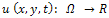
In this section, we review some basic mathematical concepts of the nonlinear diffusion PDEs proposed by Perona and Malik[1]. Let be the grayscaled intensity image with a diffusion time t, for the image domain.

The nonlinear PDE equation is given by:

(1)

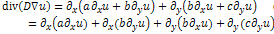
where denotes the first derivative regarding the diffusion time t; denotes the gradient modulus and g(.) is a non-increasing function, known as the diffusivity function which allows isotropic diffusion in flat regions and no diffusion near edges.

By developing the divergence term of (1), we obtain:

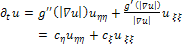(2)

Where: and are respectively the second spatial derivatives of in the directions of the gradient, and its orthogonal ; H denotes the Hessian of u. According to these definitions, on the image discontinuities, we have the diffusion along (normal to the edge) weighted with and a diffusion along (tangential to the edge) weighted with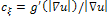. To understand the principle of the anisotropic diffusion, let represent a contour C (figure 1) separating two homogeneous regions of the image, the isophote lines (e.g. level curves of equal gray-levels) correspond to u(x,y) = c. In this case, the vector is normal to the contour C, the set is then a moving orthonormal basis whose configuration depends on the current coordinate point (x, y). In the neighborhood of a contour C, the image presents a strong gradient. To better preserve these discontinuities, it is preferable to diffuse only in the direction parallel to C (i.e. in the -direction). In this case, we have to inhibit the coefficient of (e.g. ), and to suppose that the coefficient of does not vanish.

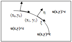Figure 1. Image contour and its moving orthonormal basis

So it appears the following conditions for the choice of the g( ) functions to be an edge preserving :

 :avoids inverse diffusion

:allows isotropic diffusion for low gradient.allows anisotropic diffusion to preserve discontinuities for the high gradient.

An extension of the nonlinear diffusion filtering to vector-valued image (e.g. color image) has been proposed [20][3]. It evolves: under the diffusion equations:

Where: denotes the i^th component channels of

Note that, represents the luminance function, which coupled all vectors channels taking the strong correlations among channels. However, this luminance function is not being able to detect iso-luminance contours.

3. Non Linear Diffusion Tensor

The non linear diffusion PDE saw previously does not give reliable information in the presence of flow-like structures (e.g. fingerprints). It would be desirable to rotate the flow towards the orientation of interesting features. This can be easily achieved by using the structure tensor, also referred to the second moment matrix. For a multivalued image, the structure tensor has the following form:

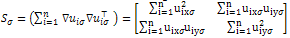(4)

With: the smoothed version of the gradient which is obtained by a convolution with a Gaussian kernel. The structure scale determines the size of the resulting flow-like patterns. Increasing gives an increased distance between the resulting flow lines.

These new gradient features allow a more precise description of the local gradient characteristics. However, it is more convenient to use a smoothed version of, that is:

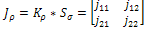(5)

Where: a Gaussian kernel with standard deviation.The integration scale averages orientation information. Therefore, it helps to stabilize the directional behavior of the filter. In particular, it is possible to close interrupted lines if is equal or larger than the gap size. In order to enhance coherent structures, the integration scale should be larger than the structure scale (. In summary, the convolution with the Gaussian kernels,make the structure tensor measure more coherent. To go further into the formalism, the structure tensor can be written over its eigenvalues ()and eigenvectors(), that is:

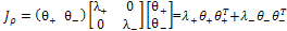(6)

The eigenvectors of give the preferred local orientations, and the corresponding eigenvalues denote the local contrast along these directions.

The eigenvalues of are given by :

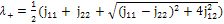(7)

(8)

And the eigenvectors satisfy :

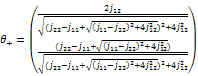(9)

and.

The eigenvector which is associated with the larger eigenvalue defines the direction of largest spatial change (i.e. the “gradient” direction). There are several ways to express the norm of the vector gradient to detect edges and corners; the most used is .The eigenvalues are indeed well adapted to discriminate different geometric cases:

If , the region doesn't contain any edges or corners. For this configuration, the variation norm should be low.

If, there are a lot of vector variations. The current point may be located on a vector edge. For this configuration, the variation norm should be high.

If, there is a saddle point of the vector surface, which can possibly be a vector corner in the image In this case should be even higher than the case above.

We note that for the case of the scalar image (e.g. n=1), 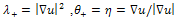and

Moreover, Weickert [3] proposed a non linear diffusion tensor by replacing the diffusivity function g(.) in (1) with a structure tensor, to create a truly anisotropic scheme, that is:

(10)

Where is the diffusion tensor which is positive definite symmetric 2x2 matrix. This tensor possesses the same eigenvectorsas the structure tensor and uses λ₁ and λ₂ to control the diffusion speeds in these two directions, that is:

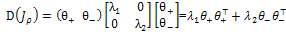(11)

The Diffusion tensor D takes the form of an ellipsoid as is represented in figure 2. We note that for the scalar image from (1), the diffusion tensor is reduced to ; where I_d : Identity matrix.

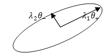Figure 2. Diffusion tensor 2D representation

In the coherence enhancing diffusion (CED) proposed by Weiker [4], the eigenvalues are assembled via:

(12)

Where and.

In flat regions, we should have and then 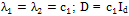where Id is the identity matrix. The tensor D is defined to be isotropic in these regions and takes the form of a circle of radius.

Along image contours, we have, and then . The diffusion tensor D is then anisotropic, mainly directed by the smoothed direction of the image isophotes.

The idea from the CED approach is that broken boundries of a single structure could be reconnected by allowing diffusion along the orientation of greatest coherence

4. Proposed Method

Our idea is to combine two types of tensors: one allows diffusion along the orientation of greatest coherence, while the other allows diffusion along orthogonal directions. It is viewed as a regularization process. The proposed equation is as follows:

The parameter can be viewed as a parameter of regularization which ensures the compromise between the two tensors. The tensor is derived from (11), that is = with the following diffusion weight functions:

(13)

The tensor D₂ is constructed from the local coordinates system . For a scalar image, the tensor D₂ takes the form:

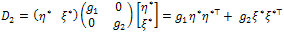(14)

: denote the local coordinate system which are the smoothed version of; with:

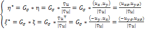(15)

Where: denotes a Gaussian Kernel; and

.

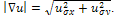By developing (14), the tensor D₂ can be expressed by:

Where : denote the conductivity in the direction of the gradient and along the isophotes respectively. There are several choices for these conductivities, the wise choice is: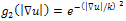and 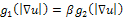, with . This allows preserving and enhancing edges while smoothing within flat regions. Indeed, when the gradient modulus is high (e.g. edges, corners region), both tends to 0, inhibiting the effect of diffusion_. In contrast, when is low (e.g. flat region), tends to two constants: 1 and respectively, the diffusion is isotropic in ()directions. The extension of (16) to multivalued (e.g. color) images require the integration of the spectral components, that is:

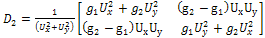(17)

With:

Furthermore, equation (12) can be solved numerically using finite differences [2]. The time derivative is approximated by the forward difference, which leads to the iterative scheme:

(18)

The divergence term is approximated using symmetrical central differences, that is:

(19)

Where: the tensor term (i.e. D₁, D₂),

And: the central differences of any F functions.

The main steps of the algorithm are:

The algorithm has been implemented with Matlab language. In the following section, we will give some experimental results.

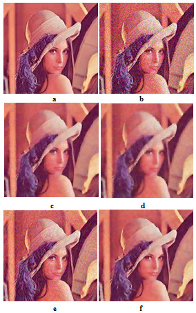Figure 3. Comparison results;-a- Original image,-b- Degraded image,-c- Total Variation (TV) method,-d- Bilateral Filter (BF) method,-e- CED method,-f- Proposed method

5. Experimental Results

We test the performance of the proposed algorithm with the famous “Lena” image sized 256x256 pixels figure 3-(a). A white gaussian noise with SNR=7.27 dB is added to the original image to obtain the noisy version showed in figure 3(b).The model’s parameters are fixed to: N = 10, . The restored image in figure 3-f shows a significantly improvement, edges and discontinuities have been recovered and preserved with a good suppression of noise. Compared to the other methods, we note that the TV one (figure 3(c)) has similar performance.

Nevertheless, our method seems to better preserve and enhance discontinuities. The CED method (figure 3(e)) is efficient preserving details, but introduces artifacts and streamlines in flat regions. The BF method is efficient removing noise, but loses details. To evaluate and quantify the quality image, we use two measures: the classic peak signal-to-noise-ratio (PSNR) and the mean structural similarity (MSSIM) index [15], which compares the structure of two images after subtracting luminance, and normalizing variance. The MSSIM approximates the perceived visual quality of an image better than PSNR. It takes values in [0,1] and increases as the quality increases. Table 1 confirms the effectiveness of our model with the highest score of MSSIM.

Table 1. Quantitative assessment comparison Methods PSNR(dB) MSSIM TV 28.07 0.85 Bilateral Filter 27.71 0.76 CED 26.06 0.61 Proposed 28.10 0.86

Figure 4. shows the performance of the algorithm on a real photographic JPEG image acquired from the Web site.

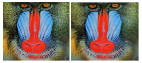Figure 4. Results on a real photographic image, -a- Original image, -b- Restored image

It can be observed that the restored image seems to be sharper, less noisy, and having a good edges and color preservation.

6. Conclusions

In this paper, we have proposed a new approach for image denoising based on the diffusion tensors. The idea is to combine two types of tensors: one allows diffusion along the orientation of greatest coherence, while the other allows diffusion along orthogonal directions. This is offering a flexible and effective control on the diffusion process. Experimental results on test and real digital pictures are very promising and provide very good quality images in terms of noise reduction and discontinuities preservation. Future work will include automatic parameters estimation and computational models that can automatically predict perceptual image quality.