1. Introduction

1.1. Artificial Neural Networks (ANN)

A neural network is a computing paradigm that is loosely modelled after cortical structures of the brain. It consists of interconnected processing elements called neurons that work together to produce an output function. The output of a neural network relies on the cooperation of the individual neurons within the network to operate.

Processing of information by neural networks is often done in parallel rather than in series. Neural network is sometimes used to refer to a branch of computational science that uses neural networks as models to either simulate or analyze complex phenomena and/or study the principles of operation of neural networks analytically.

The optical character recognition is one of the earliest applications of Artificial Neural Networks. Classical methods in pattern recognition do not as such suffice for the recognition of visual characters[1]. Because the ‘same’ characters differ in sizes, shapes and styles from person to person or time to time with the same person. And shapes of characters may be more noisy in different handwritings. ANN confirms adaptive learning by using previous samples and gains generalization capability. A neural system is able to work with noisy, unknown and indefinite data. Other advantages include:

1. Adaptive learning: An ability to learn how to do tasks based on the data given for training or initial experience.

2. Self-Organization: An ANN can create its own organization or representation of the information it receives during learning time.

3. Real Time Operation: ANN computations may be carried out in parallel, and special hardware devices are being designed and manufactured which take advantage of this capability.

4. Fault Tolerance via Redundant Information Coding: Partial destruction of a network leads to the corresponding degradation of performance. However, some network capabilities may be retained even with major network damage.

Neural networks take a different approach to problem solving than that of conventional computers.

Conventional computers use an algorithmic approach i.e. the computer follows a set of instructions in order to solve a problem. Unless the specific steps that the computer needs to follow are known the computer cannot solve the problem. That restricts the problem solving capability of conventional computers to problems that we already understand and know how to solve. But computers would be so much more useful if they could do things that we don't exactly know how to do. Neural networks process information in a similar way the human brain does. The network is composed of a large number of highly interconnected processing elements (neurons) working in parallel to solve a specific problem. Neural networks example. They cannot be programmed to perform a specific task. The examples must be selected carefully otherwise useful time is wasted or even worse the network might be functioning incorrectly. The disadvantage is that because the network finds out how to solve the problem by itself, its operation can be unpredictable.

Neural networks are a form of multiprocessor computer system, with i) simple processing elements, ii) a high degree of interconnection, iii) simple scalar messages, & iv) adaptive interaction between elements. Conventional computers use a cognitive approach to problem solving; the way the problem is to solved must be known and stated in small unambiguous instructions. These instructions are then converted to a high level language program and then into machine code that the computer can understand. These machines are totally predictable; if anything goes wrong is due to a software or hardware fault. Neural networks and conventional algorithmic computers are not in competition but complement each other. There are tasks are more suited to an algorithmic approach like arithmetic operations and tasks that are more suited to neural networks. Even more, a large number of tasks, require systems that use a combination of the two approaches (normally a conventional computer is used to supervise the neural network) in order to perform at maximum efficiency.

2. Basic Study: The Biological Model -How the Human Brain Learns

The brain is principally composed of a very large number (circa 10,000,000,000) of neurons, massively interconnected (with an average of several thousand interconnects per neuron, although this varies enormously). Each neuron is a specialized cell which can propagate an electrochemical signal. The neuron has a branching input structure, a cell body, and a branching output structure (the axon). The axons of one cell connect to the dendrites of another via a synapse. When a neuron is activated, it fires an electrochemical signal along the axon. This signal crosses the synapses to other neurons, which may in turn fire. A neuron fires only if the total signal received at the cell body from the dendrites exceeds a certain level (the firing threshold).

Recent research in cognitive science, in particular in the area of no conscious information processing, have further demonstrated the enormous capacity of the human mind to infer ("learn") simple input-output covariations from extremely complex stimuli. Thus, from a very large number of extremely simple processing units (each performing a weighted sum of its inputs, and then firing a binary signal if the total input exceeds a certain level) the brain manages to perform extremely complex tasks. Of course, there is a great deal of complexity in the brain is interesting that artificial neural networks can achieve some remarkable results using a model not much more complex than this. Much is still unknown about how the brain trains itself to process information, so theories abound. In the human brain, a typical neuron collects signals from others through a host of fine structures called dendrites. The neuron sends out spikes of electrical activity through a long, thin stand known as an axon, which splits into thousands of branches. At the end of each branch, a structure called a synapse converts the activity from the axon into electrical effects that inhibit or excite activity from the axon into electrical effects that inhibit or excite activity in the connected neurons. When a neuron receives excitatory input that is sufficiently large compared with its inhibitory input, it sends a spike of electrical activity down its axon. Learning occurs by changing the effectiveness of the synapses so that the influence of one neuron on another changes

2.1. Structure of a Neuron

There are many different types of neuron or cells. A typical cell has three major region; the cell body, the axon and the dendrites. The dendrites receive information from neurons through axon that serves as transmission lines. An axon carries impulses from the neuron. The axon-dendrite contact organ is called synapse. In synapse the neuron introduces its signal to the neighboring neuron. The neuron respond to the total of its inputs aggregated within a short time interval, called the period of latent summation. A neuron generates a pulse response and sends it to its axon only if the necessary condition for firing fulfilled.

The condition for firing is that excitation should exceed Inhabitation by an amount called the threshold of the neuron. Characteristics of action potential propagation along axons:

1). An action potential is propagated without delay.

2). The propagation of an action potential along one axon does not interfere with other neighboring nerve fibers.

3). An axon is not easily exhausted; it can propagate many impulses for a long period of time.

2.2. From Human Neurons to Artificial Neurons

We conduct these neural networks by first trying to deduce the essential features of neurons and their interconnections. We then typically program a computer to simulate these features.

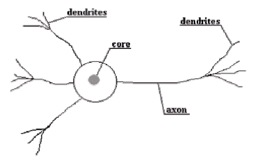Figure 1. Biological Neuron.

However because our knowledge of neurons is incomplete and our computing power is limited, our models are necessarily gross idealizations of real networks of neurons. To capture the essence of biological neural systems, an artificial neuron is defined as follows. It receives a number of inputs. Each input comes via a connection that has a strength (or weight); these weights correspond to synaptic efficacy in a biological neuron. Each neuron also has a single threshold value. The weighted sum of the inputs is formed, and the threshold subtracted, to compose the activation of the neuron. The activation signal is passed through an activation function to produce the output of the neuron. If the step activation function is used (i.e., the neuron's output is 0 if the input is less than zero, and 1 if the input is greater than or equal to 0).

A neural network has its neurons divided into subgroups of fields and elements in each subgroup are placed in a row or a column. Each subgroup is then called to as layer of neurons in the network. A neural network may have input layer that supply the input signals for the neurons in the next layer, output layer where output is generated and in between them hidden layer(s) that process information between input and output layers. Two neurons are connected with a weight which may be positive, negative, or zero. Basically, the internal activation or raw output of a neuron in a neural network is a weighted sum of its inputs multiplied by weights connected to it.

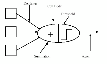Figure 2. The neuron model.

In mathematical form Y =W_i X_i where, Y is the activation (output); W_i, the i^th weight of i^th neuron; and X_i; is the i^th input to i^th neuron. activation function to produce the output of the neuron. When the entire network has been executed, the outputs of the output layer act as the output of the entire network.

2.3. Structure of a Neuron[2]

There are many different types of neuron or cells. A typical cell has three major region; the cell body, the axon and the dendrites. The dendrites receive information from neurons through axon that serves as transmission lines. An axon carries impulses from the neuron. The axon-dendrite contact organ is called synapse. In synapse the neuron introduces its signal to the neighboring neuron. The neuron respond to the total of its inputs aggregated within a short time interval, called the period of latent summation. A neuron generates a pulse response and sends it to its axon only if the necessary condition for firing fulfilled. The condition for firing is that excitation should exceed Inhabitation by an amount called the threshold of the neuron.

Characteristics of action potential propagation along axons:

1). An action potential is propagated without delay.

2). The propagation of an action potential along one axon does not interfere with other neighboring nerve fibers.

3). An axon is not easily exhausted; it can propagate many impulses for a long period of time.

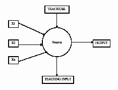Figure 3. A simple Neuron.

3. Training of Artificial Neural Network

A network is trained so that application of a set of inputs, produce the desired (or, at least consistent) set of outputs. Each such input set is referred to as vector. Training is accomplished by sequentially applying input vectors, while adjusting network weights according to a predetermined procedure. During training the network weights gradually converge to values such that each input vector produces the desired output vector.

3.1. Supervised Training

This training requires the pairing of each input vector with a target, representing the ‘” desired output. Together these are called a training pair. Usually a network is trained over a number of such training pairs. An input vector is applied, the output of the network is compared with the corresponding target vector and the difference (error) is feed back through the network and weights are adjusted according to the algorithm that leads to minimize the error. The vectors of the training set are applied sequentially, and error are calculated and weights adjusted for each vector, until the error for the entire training set is an acceptably low level.

3.2. Unsupervised Training

“It requires no target vector for the outputs and hence no comparison to “predetermined ideal response. The training set consists solely of input vectors. The training algorithm modifies the network weights to produce output vectors that are consistent, that is both application of one of the training vector or application of a , vector that is sufficiently similar to it, will produce the same pattern of outputs. The training process, therefore extracts the statistical properties of the training set and groups similar vectors into classes.

4. Pattern Recognition and Neural Networks

Pattern classification deals with the identification or interpretation of the pattern in an image. It aims to extract information about the image and/or classify its contents. For some simple and frequently encountered patterns, the recognition process can be a straight forward task. However when the patterns are complex or when pattern characteristics cannot be predicted beforehand, then one needs a high-level system to perform pattern classification.

4.1. Required Steps for Pattern Recognition[5]

In general, the following steps are involved in pattern recognition

a). Image representation: In image representation one is concerned with the characterization of the quantity that each pixel represents. The sampling rate (number of pixels per unit area) has to be large enough to preserve the useful information in the image.

b). Image segmentation: Image segmentation refers to the decomposition of the image into its components. It is basically done to identify regions in the image which have uniform brightness, color and texture. It is a key stepping in image analysis. For example, a document reader must first segment the various characters before proceeding to identify them. In binary images i.e., images in which the pixels have values of either 1 or 0, the segmentation process is relatively simpler.

c). Feature Extraction: The ultimate aim in large number of applications is to extract important features from the image data. It is a process of converting the pixel-map representation of the input image into a group of quantitative descriptors called feature values.

d). Classification: After the adequately required features are extracted, the object is cla~sified under one of many standard classes. It is here that the Artificial Neural Network is used to do the classification.

5. Conventional Techniques

Conventional techniques used for printed characters consisted of scanning the printed character, sampling and quantization into two levels 0 and 1, to produce a binary matrix of N x N for each printed character. This binary matrices are then matched with standard character matrices, to identify to which character class, the given test character belongs.

In conventional techniques for handwritten characters required the writer to write the character in a preprinted rectangular grid, invisible to the scanning systems. But this system limits the domain of the usage of such systems, because the grid system becomes system dependent.

Hence to overcome the difficulties of free format hand print recognition, many techniques are adopted. Segmentation (approximating by straight lines) characters Into shorter units, has been commonly used technique.

5.1. Methodology Developed

The basic methodology developed in the project by us for the purpose of handwritten character recognition is depicted below.

Preprocessor Block

a) Noise removing

b) Skeletonization

c) Normalization

The function of this module is to remove noise by applying various digital image processing techniques and the image is normalized into 32x32 pixels. The output is a 32x32 pixels binary image of the character. Skeletonization refers to remove extra pixels and get only skeleton of character. In this paper, mouse has been initialized in graphics mode and samples have been taken directly on the screen by various students and faculty members. A 32x 32 box has been created on screen and users are supposed to write in the box with the help of mouse. The samples taken on the screen are converted into three formats: 0 and 1 format, Gradients format and 12 directional feature formats. These three formats have been stored in three different files and taken as input to the network.

5.2. Character Matrix Quantization

In application like digit recognition, the normalized character matrix, which usually has a size of 8 x 8 pixels, can be directly fed to the neural network for recognition. But as the number of pattern classes increases, the matrix size increases and so does the number of input neurons. To increase the efficiency of the neural network, the number of input and hidden layers increases. This, in turn has the effect of significantly increasing the training time of the neural network. Therefore Instead of feeding the Os and 1s directly, the character matrix is quantified (encoded) by simply breaking it into many smaller N x N grids. The encoding in floating point vectors is accomplished by dividing number of 1s in the grid by total number of bits in it. The set of floating numbers are fed as input vectors to the neural network.

The quantization too is a trade-off between accuracy and complexity of neural network structure. Larger the size of quantizing grids, smaller the input vector and training time. Accuracy suffers in this case, because of masking of certain important features in the pattern by the large sized grids. Smaller the size of the grid, better is the accuracy, but the neural network structure blows up and so does the training period required.

For the present Implementation scheme, the quantization grid of 2 x 2 seems to be good choice, without much loss of accuracy. Hence 10 x 10 (100) floating point numbers from the input vector of a character are fed to the neural network.

5.3. Back-Propagated Neural Network for Recognition

The feed forward back-propagation network is a very popular model in neural network. It does not have feedback connections, but errors are back-propagated during training. Least mean squared error is used. Many applications can be formulated for using a feed forward back-propagation network. Errors in the output determine measures of hidden layer output errors, which are used as a basis for adjustment of connection weights between the pairs of layers and recalculating the outputs is an Iterative process that is carried on till the errors fall below a certain tolerance level. Learning rate parameters scale the adjustment to the weights[6].

The back-propagation algorithm (BPA), also called the generalized delta rule, provides a way to calculate the gradient of the error function efficiently using the chain rule of differentiation. The error after initial computation in the forward pass is propagated backward from the output units, layer by layer, justifying the name "back-propagation"[4].

Let the training set be {x(k), d(k)} where k = 1 to Nand x(k) is the input pattern vector to the network and d(k) is the desired output vector for the input pattern x(k). the output of the jth output unit is denoted by yj. Connections weights from the jth unit, In one layer, to the jth unit, in the layer above, are denoted by W (/) .The superscript I denotes the fact that the layer I containing the jth unit is I layers below the output layer. When I = 0, the output superscript is omitted.

Let m be the number of output units. Suppose that dj(k) is the desired output from the jth output unit whose actual output in response to the kth input pattern x(k) is yj, for j = 1,2,3 ,m. Define the sum of squares of the error over all output units for this kth pattern by 1 In 2 ~ E (k) = iL [Y j (k) -d .j (k)] (4..1) and the total classification error over the set of N patterns by N E r = L E (k) (4.2) *=1

In Eq. (4.1), the constant multiplier of value '12 does not influence the minimization but has been inserted for convenience in representation following the gradient calculation. The process of computing the error E(k) in Eq. (4.1) is called a forward. After presentation of a training pattern x(k), the classification error can be computed. The objective is to determine how the error is reducible by the adjustment network parameters. How the error E(k) is affected by the output from unit j at the output layer is determined easily from Eq. (4.1) by computing oE(k)ay; = Y i -d I (4.3)

The net input to unit j in the output layer is given by: (I) S j = L Y i W!i (4.4)

where y ~ I) is the output from the Ith unit in the first layer below the output layer, wij is the connection weight multiplying y :') .

1. Let A be the number of units in the input layer, as determined by the length "" of the training Input vectors. Let C be the number of units in the output layer. "" Now choose B, the number of units in the hidden layer.( "successfullarge scale" networks have used topologies like 203-80-26 [Sejnowski and Rosenberg, 1987], 960-9-45 [Pomerleau,1989]. ; a larger hidden layer results in a mor powerful network, but too much power may be undesirable). The input and -hidden layers each have an extra unit used for thresholding. We denote the "" activation levels of the units In the Input layer by xj , In the hidden layer by hi, and In the output layer by oj. Weights connecting the input layer to the hidden layer are denoted by wlij, where the subscript I indexes the input unit -, and j indexes the hidden units. Likewise, weights connecting the hidden layer --to the output layer are denoted by w2ij, with i indexing to hidden units and j "" indexing output units.

2. Initialize the weights in the network. Each weight should be set randomly to a number between -1 and +1.8 Wlij = random (-1, +1) for all i = 0 A, j = 1 B W2ij = random (-1, +1) for all i = 0 B, j = 1 ...,... C

3. Initialize the activations of the thresholding units. The values of these thresholding units should never change.

Xo = 1.0

ho = 1.0'

4. Choose an input-output pair. Suppose the input vector is xi and the target --output vector is yi. Assign activation levels to the input units.

5. ~ropagate the activations from the units in the input layer to the units in the '"'" hidden layer using the activation function as

The algorithm generalizes straightforwardly to networks of more than three layers. For each extra hidden layer, insert a forward propagation step between steps 6 and 7, an error computation step between steps 8 and 9, and a adjustment step between steps 10 and 11. Error computation for hidden units should use the equation in step 8, but with i ranging over the units in the next layer.

The speed of learning can be increased by modifying the weight modification steps 9 and 10 to include a momentum term f3.

6. Conclusions

The BPN network designed proposed has the ability to recognize stimulus patterns without affecting by shift in position not by a small distortion in shape of input pattern. It also has a function of organization, which processes by means of Supervised Learning. If a set of input patterns are repeatedly presented to it, it gradually acquires the ability to recognize these patterns. It is not necessary to give any instructions about the categories to which the stimulus patterns should belong. The performance of the network has been demonstrated by simulating on a computer. We do not advocate that the network is a complete model for the mechanism of character recognition in the brain, but we propose it as a working design for some neural mechanisms of visual pattern recognition. It is conjectured that, in the Human Brain the process of recognizing familiar patterns such as alphabets of our native Language differs from that of recognizing unfamiliar patterns such as foreign alphabets, which we have just begun to learn. The design of information processing proposed in this project is of great use not only as an inference upon the mechanism of brain but also to the field of Engineering. One of the largest and longstanding difficulties is in designing a pattern recognizing machine has been the problem how to cope with the shift in position and the distortion in the shape of the input patterns. The network proposed in this paper gives a partial solution to this difficulty. This principle can also be applied to auditory information processing such as Speech Recognition.