1. Introduction

Computational Grid (CG) is an aggregation of hardware and software resources that provides dependable, consistent, pervasive and inexpensive access to high end computational facilities despite the geographical distribution of both resources and the users. It primarily satisfies the computational requirements of the job. Users or the participants of the grid lie at one end of the grid that may demand the execution of a job through an intelligent interface. At the other end lies the pool of registered resources in the grid and the grid middleware searches appropriate resources for the job execution. Depending on the execution policies and the job’s requirement, the job will eventually be scheduled on one of the suitable resource i.e. clusters (consisting of various computing nodes). Thus, the grid users visualize the grid as an enormous source of computing energy that facilitates the execution of any type of job efficiently on the suitable resources of the grid.

Usually there are two types of jobs; fine grain and coarse grain. Objectives of fine grain jobs are to exploit the parallelism, whereas coarse grain jobs exploit the distribution. Grid is suited for both types of jobs. It has been observed that during the job execution over the period of time, nodes of the grid become highly imbalance which may result in the performance degradation of the grid. In order to keep the grideffective and efficient, load balancing is imperative. Load balancing is the act that insures even distribution of computational load on various nodes of computational grid. Load balancing[1] means spreading the computation evenly across the nodes while optimizing the inter process communication. To achieve load balancing for fine grain jobs is very difficult, though it is nontrivial even for the coarse grain jobs. Thus, load balancing is a fundamental issue in order to utilize the grid nodes and achieve high performance in computational grid.

GA[2,3], is often used to solve the problem in which possible solution involves searching a big search space of potential solutions. The problem, being addressed in this work, is the load balancing in computational grid that also has a big solution search space. GA has been applied to solve this problem. So far, very few work with sole objective of load balancing, particularly in computational grid, has been done. In[4], a model for very small grid and work load has been suggested. In[5], static load balancing is done which is unrealistic in real world grid. This paper proposes a realistic model for load balancing for a reasonably larger computational grid. In[6], load balancing in cluster is suggested. In[7], hybrid load balancing strategy of sequential jobs for grid computing environments is suggested. In[8], based on average response time, novel load balancing algorithm for computational grid is discussed. In[9], decentralized recent neighbor load balancing algorithm for Computational Grid is discussed. In[10], analyzing load balance term-based partition for parallel system is discussed.

The organization of this paper is as follows. After the introduction in section 1, the problem has been elaborated in section 2. GA based load balancing model has been proposed in section 3. Performance evaluation through experiment and observation there from has been given in section 4. Finally, concluding remarks appear in section 5.

2. The Problem

Grid is essentially a heterogeneous collection of computational and non computational resources. This heterogeneity introduces many related challenges that include diversity in terms of local resources, dynamic nature of the local resources, creation and management of services and maintaining the load. Efficient job execution on the grid depends on the proper scheduling and load balancing on such system.

Load, in particular, is defined as the total computational workload assigned to any computational node. Load balancing[4] is the technique to re-distribute the workload evenly across the nodes in the grid environment. It is required in order to achieve the optimal resource utilization in the grid system. With proper load balancing other Quality of Service (QoS) parameters[11,12], e.g. throughput, system utilization etc. is also optimized.

Load balancing is a problem that arises in parallel and distributed system and in grid. Modern computational grid is being used not only as a distributed system but also for parallel job execution. So grid is suited for both types of jobs; fine grain and coarse grain. When the jobs are coarser, better load balancing often may not be possible. With fine grain jobs, load balancing can be properly achieved. Though, for both types of job, it is a computationally complex problem.

As discussed, load balancing is the process of evenly distributing the job on the computational resources of the grid. Grid, being a dynamic system, often leaves vacuum after some period of time as there might be some incoming jobs and some exiting the system. Load balancing strategy also deals with the migration of the jobs periodically from one node to another in order to balance the workload amongst the grid nodes. Therefore, it is a computationally hard problem and falls in the NP class problem[13]. GA[4,14,15] is used to solve dynamic load balancing problem in parallel/distributed system and the grid. The mapping techniques of load balancing for parallel system are discussed in literature[16,17,18]. The load balancing and a data flows are described in[19]. The load balancing for distributed system is described in[20,21,22]. The load balancing in grid is discussed in literature[4,5]. Tree based load balancing in grid is discussed in the literature[4,5,23,24].

3. The Proposed Model

The work, proposed here, has been derived from the work of[4,5], with some modifications. It suggests necessity of quantification of load in order to achieve load balancing in computational grid. Quantification of the load is done and the objective function is derived based on the load distribution on the computational nodes.

3.1. The Objective Function

The objective is derived on the basis of the load variation in each node in computational grid environment. In ideal case i.e. when the load is evenly distributed among the nodes in the grid environment, load variation is zero. But often it may not be possible. Therefore, load variation is minimized to its fullest possible extent. In order to calculate the load variation amongst the grid nodes, first the average load in the grid is calculated and thus, it is required to calculate the total load. Load on the grid node is computed based on the size of the job module. The average load () on grid, can be computed using total load () in the grid and number of nodes in the grid (m). The calculations are as follows.

At any i^th node, weight is obtained as given in Equation 1.

(1)

Where, r is the numbers of modules allocated to the i^th node, and is module size.

For m nodes, total load in computational grid environment is computed as follows.

(2)

Average load in computational grid environment is obtained as follows.

(3)

Thus, the objective function is derived as follows.

(4)

In above Equation is the load (weight) at the j^th node.

Equation 4 depicts the overall load variation in computational grid environment. Objective is to minimize this value to get the optimal load distribution.

3.2. The Model

The proposed model uses GA to minimize the load variation in order to achieve better load balancing. GA based load balancing model has various problem specific modules. These are discussed as follows.

Chromosome Structure: Chromosome represents the solution to the problem and it varies from problem to problem. The genes of the chromosome, used in the model, contains task associated with the machine. Its structure is as below[25,26].

Struct chromosome {task[]; machine ;};

Structure of the task and the machine is as follows.

Struct task {int task_ no; double task size ;} task;

Struct machine {int machine no; double machine ;} machine;

Initial Population: Number of chromosome form the population. In the model, each chromosome of the population is generated randomly. The random generation is based on the random permutation concept.

Crossover & Mutation: Two children are generated from two parent chromosomes in the crossover operation. The proposed model uses uniform crossover. Uniform crossover randomly generates a binary mask of zeroes and ones [25,26]. Using that mask, we perform the crossover. The probability of applying crossover is 0.95. In mutation, the random flip occurs in some bits in genetic population. Mutation is used with probability 0.05.

Selection: Selection is based on the sorting. Population is sorted based on the fitness values using sorting algorithm. Best half of the population is selected after every generation.

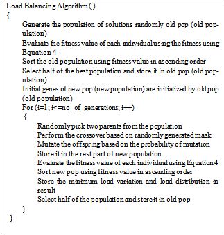
3.3. The Algorithm

Proposed model schedules the jobs on the grid with the objective to minimize the load variation. It means it takes the best schedule which has minimum load variation. There are various inputs to the problem. These are number of tasks, number of machines, population size and the number of generation up to which the algorithm has to execute. Initial population of the chromosome is randomly generated[25,26]. Tasks are also randomly generated with the range of the task size. The total load on grid is calculated by taking the summation of the task size in the grid as given in Equation 2. The average load on the grid is obtained using Equation 3. To generate initial population, tasks are randomly distributed to the nodes of the grid. Equation 4 is used to compute the fitness of the old population. A uniform crossover[25] is applied in this model. Mutation[25] is also effectuated sometimes with the probability 0.05. The whole process is repeated until the stopping criterion is met.

Table 1. Pseudo-code for Load Balancing Algorithm using GA.

The algorithm for load balancing, in the proposed model, is based on GA. Pseudo-code for the algorithm is given in table 1.

4. Performance Evaluation

Performance of the proposed model is evaluated by its simulation. Simulation program is written in C++. In most of the experiment, it has been observed that the solution converges by 200 generations. Other considered parameters for experiment are as follows.

Simulation Parameters: The input parameters, used in the experiment, are as follows.

Range of number of machines are 20 to 100 in every experiment, Population Size is 50, Number of jobs are 100, Generation to run the experiment is 200, Load ranges vary to depict fine grain and coarse grain jobs and is shown in the experiment.

4.1. Experiment 1

In this experiment, we have considered fixed range of the load with modules in the size of 100-200 Mflops. Number of machines vary and is consists of 20, 40, 50, 60, 80,100 nodes with total load on the grid as 15074 Mflops. These are considered to be fine grain modules. Load variation (in Mflops) is depicted on Y-axis for number of generations (X-axis) in Figures 1 and 2.

Figure 1. Load Balancing Observation for fine grain jobs.

Figure 2. Load Balancing Observation for fine grain jobs.

The following observations are derived from Figures 1 and 2.

Solution converges by 170 generations. When the number of nodes increases, load variation decreases e.g. for 40 nodes the load variation is 359.333 which becomes 220.541 for 60 nodes and further 152.446 for 80 nodes. It reflects that load distribution is better when the number of nodes is more in the grid.

Figure 3. Load Distribution for 20 nodes.

Figure 4. Load Distribution for 40 nodes.

Figure 5. Load Distribution with 50 Nodes.

Figure 6. Load Distribution with 60 Nodes.

Optimal load distribution with respect to various nodes has been depicted in the graphs in Figures 3 to 8. Y-axis represents the load in Mflops and X-axis represents the node number in the grid. Other input parameters are same as of the above experiment.

Graph in Figure 4 shows the distribution of the load on the grid consisting of 40 nodes. Similar type of experimentation has been done with 50, 60, 80 and 100 nodes in the grid. The graphs are depicted in the Figures 5 to 8.

Figure 7. Load Distribution with 80 Nodes.

Figure 8. Load Distribution with 100 nodes.

The following observations are derived from Figures 3 to 8.

All the graphs show that a better load balancing is achieved as none are very few nodes are sitting idle. If the number of nodes is increased in the grid, load distribution is better. The modules are fine grain therefore the better load distribution is observed.

4.2. Experiment 2

In experiment 2, the range of module size has been increased i.e. from fine grain modules to coarser grain modules. Load is in fixed range (200-300) with fixed modules (100) but number of machines varies i.e. 20, 40, 50, 60, 80, 100 nodes with total load on grid 24749.3 Mflops that is lesser fine grain modules than experiment 1.

We study here load variation and load distribution for varying nodes. This is to observe, how the model performs on different size grid. Load variation (in Mflops) is depicted on Y-axis for number of generations (X-axis) in Figures 9 and 10.

Following observations are derived from the above experiment.

Solution converges by 170 generations. As observed from Figure 9 and 10, when the number of nodes increases, load variation decreases. It reflects that load distribution is better when the number of node is more in the grid. The modules are less fine grain than experiment 1 therefore load variation is less apart than experiment 1 even if the numbers of nodes are increased. Meaning thereby is if the modules goes to coarser grain and number of nodes are increased then conversion is less fast than experiment 1.

Load distribution in each case has also been depicted in the graphs below. This has been done for same set of input and for the grid consisting of 20, 40, 50, 60, 80 and 100 nodes. Optimal load distribution with respect to various nodes has been depicted in the graphs below. Y-axis represents the load in Mflops and X-axis represents the number of nodes in the grid.

Figure 9. Load Balancing Observation fine grain jobs.

Figure 10. Load Balancing Observation fine grain jobs.

Figure 11. Load Distribution with 20 nodes.

Above graph shows the distribution of the load on various nodes considering total 20 nodes in the grid. X-axis represents the node and Y-axis represents the load on each node.

Similar type of experimentation has been done with 40,50,60,80 and 100 node grid. The graphs for the same have been depicted in Figures 12 to 16.

Figure 12. Load Distribution with 40 nodes.

Figure 13. Load Distribution with 50 nodes.

Figure 14. Load Distribution with 60 nodes.

Figure 15. Load Distribution with 80 nodes.

Figure 16. Load Distribution with 100 nodes.

The following observations are derived from Figures 11 to 16.

All the graphs shows that a better load balancing is achieved as none of the nodes are sitting idle. If the number of nodes is increased in the grid, load distribution is better. The modules are less fine grain than experiment 1 therefore load distribution is not as good in comparisons to experiment 1.

4.3. Experiment 3

In experiment 3, we have increased the range of module size i.e. moving further from fine grain modules to coarser grain modules. Load is in fixed range (300-400) with fixed modules (100) and number of machine varies i.e. 20, 40, 50, 60, 80, 100 nodes with total load 35437.3 Mflops.

We study here load variation and load distribution when number of node varies. This is to observe, how the model performs on different size grid. Load variation (in Mflops) is depicted on Y-axis for number of generations (X-axis) in Figures 17 and 18.

The following observations follow.

Again solution converges by 170 generations. As observed from Fig. 17 and Fig. 18, when the number of nodes increases, load variation decreases. It reflects that load distribution is better when the number of node is more in the grid. The modules are less fine grain than experiment 2 therefore load variation is less apart than experiment 2 if the numbers of nodes are increased in this case. That is for coarser grain modules conversion is less fast than experiment 2.

Load distribution in each case has also been depicted in the graphs below. This has been done for same set of input and for the grid consisting of 20, 40, 50, 60, 80 and 100 nodes respectively. Optimal load distribution with respect to various nodes has been depicted in the graphs below. Y-axis represents the load in Mflops and X-axis represents the number of nodes in the grid.

Graph in figure 19 shows the distribution of the load on various nodes considering total 20 nodes in the grid.

Similar type of experimentation has been done with 40,50,60,80 node grid and 100 node grids. The graphs have been depicted in Figures 20 to 24.

The following observations are derived from Figures 19 to 24.

If the number of node is increased in grid then load distribution is better than the less number of nodes. For coarse grain modules, load distribution is not that good.

Figure 17. Load Balancing Observation for fine grain jobs.

Figure 18. Load Balancing Observation for fine grain jobs.

Figure 19. Load Distribution with 20 nodes.

Figure 20. Load Distribution with 40 nodes.

Figure 21. Load Distribution with 50 nodes.

Figure 22. Load Distribution with 60 nodes.

Figure 23. Load Distribution with 80 nodes.

Figure 24. Load Distribution with 100 nodes.

4.4. Experiment 4

We now have carried out the experiment fixing the number of nodes but varying the module size i.e. varying the load across the grid. Fixed number of machines with fixed modules but varying load i.e. 100-200 (15074), 200-300 (24749.3) and 300-400 (35437.3) Mflops. In this, we performed the experiment by varying the module sizes. This considers the fine and coarse grain jobs. Smaller range stands for fine grain and bigger range for coarse grain jobs.

Figure 25. Load Distribution with 20 nodes.

Figure 26. Load Distribution with 40 nodes.

Figure 27. Load Distribution with 50 nodes.

Figure 28. Load Distribution with 60 nodes.

Figure 29. Load Distribution with 80 nodes.

Figure 30. Load Distribution with 100 nodes.

Optimal load distribution with respect to various nodes has been depicted in the graphs below. Y-axis represents the load in Mflops and X-axis represents the node number in the grid. This has been done for the same set of input and for the grid consisting of 20, 40, 50, 60, 80 and 100 nodes.

The following observations are derived from Figures 25 to 30.

If the number of nodes is increased in grid then load distribution is better. In the fine grain modules load distribution is best. If we increase the range of module size i.e. moves from fine grain to coarse grain modules load distribution is not good.

4.5. Experiment 5

In this, we are studying the load variation for different load (i.e. module size) on fixed grid size. Graph for the three range of the module size showing the load variation is as below.

Figure 31. Load Balancing Observation with 80.

The observations are as follows.

Solution converges by 170 generations. From figure 31 it is conspicuous that when the module range increases, load variation also increases i.e. in the case of module range 100-200 the load variation is 152.846 which becomes 252.541 for module range 200-300 and further 364.99 for module range 300-400. It shows that load distribution in coarse grain jobs is uneven. Also for fine grain jobs, load distribution is better. If the modules are fine grain then load variation is least. Load variation is increased if module size range increased.

4.6. Experiment 6

In experiment 6, we vary the number of nodes in the grid on coarse gain module with load in the fixed range (100-500) for 100 modules. Total load in the grid comes out to be 31078.4 Mflops.

Figure 32. Load Distribution with 20 nodes.

Figure 33. Load Distribution with 40 nodes.

Figure 34. Load Distribution with 50 nodes.

Figure 35. Load Distribution with 60 nodes.

Figure 36. Load Distribution with 80 nodes.

Figure 37. Load Distribution with 100 nodes.

Optimal load distribution with respect to various nodes has been depicted in the graphs in Figures 32 to 37. Y-axis represents the load in Mflops and X-axis represents the number of nodes in the grid. This has been done for same set of input and for the grid consisting of 20, 40, 50, 60, 80 and 100 nodes.

The following observations are derived from Figures 32 to 37.

If number of nodes is increased in grid then load distribution is better. The modules are least fine grain than experiments 1 therefore load distribution is not good compared to the experiment 1.

5. Conclusions

This work deals with the load balancing in computational grid with emphasis on the observation of load variation and load distribution among the nodes in the computational grid environment. Six cases have been considered to observe the load variation and load distribution. First three are with fixed load and varying nodes for both fine grain and coarse grain module. Fourth experiment considers both load and number of nodes varying. Experiment five deals with fixed node and varying load for fine grain and coarse grain modules. Last experiment deals with the coarser grain modules having fixed load and varying nodes. It is concluded that when the number of nodes are increased, for fixed load, the distribution is better. In comparison to coarse grain modules, load distribution is better for fine grain modules for fixed number of nodes. It is because, fine grain modules gives more possibility of load distribution. Overall, proposed model achieves better load distribution for both fine grain as well as coarse grain jobs. The load distribution schemes can be incorporated with the scheduling algorithm to achieve better load balancing and therefore better system utilization.

ACKNOWLEDGEMENTS

The assistance for this work is provided by the University Grant Commission, New Delhi, India.