M. Sudheer 1, Pradyoth K. R. 1, Shashiraj Somayaji 2
1Department of Mechanical Engineering, St Joseph Engineering College, Mangaluru, Karnataka, India
2Department of Mechanical Engineering, B.M.S College of Engineering, Bengaluru, Karnataka, India
Correspondence to: M. Sudheer , Department of Mechanical Engineering, St Joseph Engineering College, Mangaluru, Karnataka, India.
| Email: |  |
Copyright © 2015 Scientific & Academic Publishing. All Rights Reserved.
Abstract
In the present study, elastic properties like Young’s modulus (E1 and E2) and Poisson’s ratio (v12 and v21) are evaluated for n different volume fractions along the material principal directions using finite element method (FEM). The standard commercial software ANSYS is adopted as a solver. These computational results are compared with the results obtained from analytical methods such as Rule of mixture, Halpin-Tsai, Nielsen and Chamis elastic models. The main objective of this paper is to compare the computational results with analytical methods to determine the best elastic properties. The study indicates that the Epoxy/Glass composite is more effective when the load is applied along the fiber direction. The FEM predicted results are in good comparison with results of analytical methods.
Keywords:
Epoxy/Glass, Elastic properties, Fiber volume fraction
Cite this paper: M. Sudheer , Pradyoth K. R. , Shashiraj Somayaji , Analytical and Numerical Validation of Epoxy/Glass Structural Composites for Elastic Models, American Journal of Materials Science, Vol. 5 No. 3C, 2015, pp. 162-168. doi: 10.5923/c.materials.201502.32.
1. Introduction
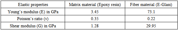
Composite materials have become essential part of today’s life because of many applications and advantages. Recently there are many researches going on in the field of engineering design and developments to improve the mechanical properties and thermal properties such as stiffness, fatigue, corrosion resistance, high stiffness to weight ratio, high strength to weight ratio, thermal resistance, etc [1]. Fiber reinforced polymer (FRP) usually made of polymer matrix reinforced by short or continuous fibers [2]. Polymer matrix usually consists of epoxy, vinyl-ester or polyester thermosetting plastic [3] because of its excellent properties and cost of material. Glass, cellulose, aramid, silicon-carbide and carbon fibers are commonly used fibers in FRP [4]. Fibers are mainly added to polymer matrix to increase the properties of strength, modulus and impact resistance. There are three factors that affect the properties of PMC are interfacial adhesion, properties of matrix, geometry and orientation of dispersed phase (fiber reinforce). Fiber reinforced polymers are commonly used in the aircraft industries, submarine, automotive, construction industries and many house old applications [1].A key factor to improve the properties of composite material is to try different possibilities such as by varying laminated martial thickness, fiber volume fraction or fiber weight ratio and fiber orientation [3, 5-7]. Designers can test for different mixing concentrations of matrix and fiber in composite lamina (varying from 0%-100% in the steps of 10%). The end results are also varied for different thickness, strength and stiffness throughout the material component. Variables such as isotropic and orthotropic materials, linear and non-linear material properties are also the essential factors.There are several methods to evaluate the mechanical properties of composite materials such as experimental, analytical and computational methods. Computational modeling and analysis method is developed drastically in these few years. Finite element method (FEM) is the one of the numerical method which is more powerful in its application in real world problems [8] and can be used to calculate elastic properties. Now, there is much commercial software available that uses finite element analysis (FEA) technique. The commercial software ANSYS is user friendly and easy to design the required model. In this paper, elastic properties of glass fiber reinforced polymer (GFRP) composite (epoxy/glass) are evaluated by creating 2D ANSYS model. Elastic properties of matrix and fiber materials for the calculations are taken from literature and are presented in Table 1 [9].Table 1. Elastic properties of matrix and fiber material [9]
 |
| |
|
2. Analytical Models
An analytical method uses various mathematical expressions to predict the elastic constants such as stiffness and strength of composite material. Different methods used evaluate the elastic properties of the composite material are Rule of mixture, Halpin-Tsai, Nielsen and Chamis method.
2.1. Rule of Mixture
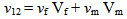
It is the simplest method to determine the elastic properties for a unidirectional composite material [1, 2]. The Young’s modulus of the matrix and fiber are taken as Em and Ef, similarly Poisson’s ratio are taken as vm and vf. If we consider length of the beam is L, then the quantities of two components inside composite in terms of volume fraction is,Longitudinal properties,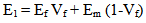 | (1) |
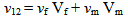 | (2) |
Where, Vf and Vm are volume fractions.Transverse properties, 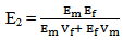 | (3) |
 | (4) |
Shear properties, | (5) |
 | (6) |
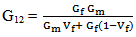
2.2. Halphin-Tsai Equation
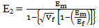
The Halpin-Tsai equation developed as a semi-empirical model to produce more complicated results on transverse Young’s modulus and longitudinal shear modulus [1].  | (7) |
where, | (8) |
in which, P = Composite material modulus E2, G12Pf = Composite fiber material modulus Ef, Gf and vfPm = Composite matrix material modulus Em, Gm and vm and ζ is an empirical factor, which measures fiber reinforcement of the composite material that depends on the loading and boundary condition of the fiber geometry. Thus Halpin-Tsai equation for transverse properties is,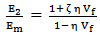 | (9) |
and | (10) |
while for longitudinal properties E1 and v12 are expressed in rule of mixture,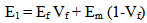 | (11) |
 | (12) |
2.3. Nielsen Elastic Model
This equation is modified from the Halpin-Tsai equation by including maximum packing fraction  . The maximum packing factor depends on geometry of the model [10].
 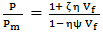 | (13) |
where, and
and 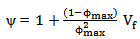 | (14) |
For a square array of fibers,  = 0.785For a hexagonal arrangement of fibers,
  = 0.907For value in between above two extremes and near the random packing,
  = 0.82.
2.4. Chamis Model
Chamis is a method modified from rule of mixture by replacing fiber volume fraction by its square root. This is most used method which gives five formulas to evaluate elastic properties [11]. 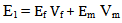 | (15) |
 | (16) |
 | (17) |
 | (18) |
Note that shear modulus G23 formula is ignored because we are comparing only the E1, E2, v12 and G12 values.
3. Finite Element Modeling
Finite element method is used to evaluate the elastic properties of epoxy/glass fiber composite material. This section contains the details of evaluation of Elastic properties such as Young’s modulus (E1 and E2), Poisson’s ratio (v12 and v21) and shear modulus (G12) along the material principal directions. To evaluate the composite material properties the commercial software ANSYS is used as ANSYS is the one of the finite element package which gives fairly good solutions.
3.1. Evaluation of Longitudinal Young’s Modulus (E11) and Major Poisson’s Ratio (ν12)
The model used is square test coupon of size 200µm and the thickness is of 20µm. Figure 1 shows geometry of test coupon for volume fraction 0.4 of glass fiber.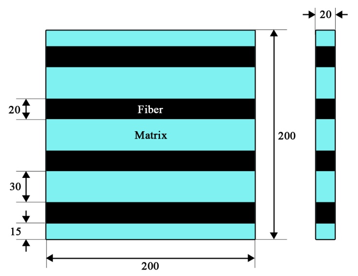 | Figure 1. Geometry of the model for evaluation of longitudinal properties (E1 and v12) |
To create a model for 0.4 fiber volume fraction, to improve the accuracy of result 426 numbers of nodes are created to generate 420 numbers of small elements. These small elements are numbered according to their material attributes. Mapped meshing was done to obtain better results.Each node has only 2 degrees of freedom (Ux and Uy) and are given along X and Y direction. Figure 2 shows loading and boundary conditions applied along X-direction to evaluate longitudinal properties E1 and v12. The boundary conditions are as follows,• The nodes on right edge BD are coupled to each other to so that they move together when the load is applied and avoid any uneven displacement.• The nodes on the left edge AC are constrained from moving in the direction ‘X’ (i.e, Ux=0).• The mid-node E located on the left edge AC is constrained from moving in the direction ‘Y’ (i.e, Uy=0).• A load of 100X10-6 N/µm2 is applied on the right edge nodes (i.e, edge BD).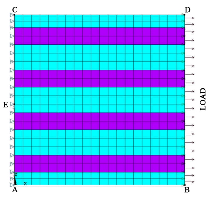 | Figure 2. Loading and boundary conditions applied along X-direction to evaluate longitudinal properties E1 and v12 |
3.2. Evaluation of Transverse Young’s Modulus (E22) and Minor Poisson’s Ratio (ν21)
The model used to evaluate transverse properties is same as the longitudinal. However transverse loading and boundary conditions are different compared to the longitudinal. The boundary conditions are as follows,• The nodes on right edge BD and nodes on left edge AC are coupled so that they move together when the load is applied.• The nodes on the bottom edge AB are constrained from moving in the direction ‘Y’ (i.e, Uy=0).• The mid-node located at the bottom edge AB is constrained from moving in the direction ‘X’ (i.e, Ux=0).• A load of 100X10-6 N/µm2 is applied on the top edge (i.e, edge CD).
3.3. Evaluation Shear Modulus (G12)
Figure 3 is used as geometry model for FEM analysis to estimate the effective shear modulus G12 for 0.4 fiber volume fraction. A square test coupon of size 200µm is placed at an angle of +45° from the X-axis. This test coupon consists of epoxy matrix and glass fiber of different elastic properties. The surrounding material is taken as a single material with combined properties of matrix and fiber. The properties of surrounding material are determined by the Rule of mixture. The surrounding material is square coupon of size 4a unit. The value of ‘a’ is calculated as  Thickness of the test coupon is taken as 20µm.
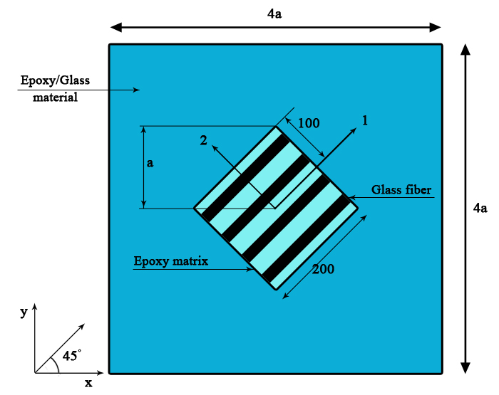 | Figure 3. Geometry of the model for evaluation of shear properties (G12) |
Figure 4 shows loading and boundary conditions applied to evaluate shear properties G12 for 0.4 fiber volume fraction. For each node has only 2 degrees of freedom (Ux and Uy) are given along X and Y direction. 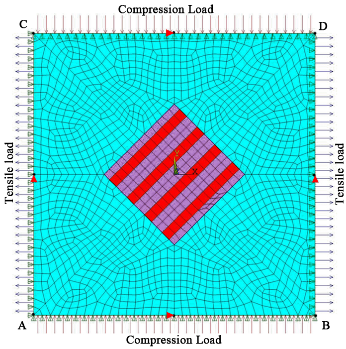 | Figure 4. Loading and boundary conditions applied on the model to evaluate shear properties G12 |
The boundary conditions are as follows,• The nodes on the bottom edge AB and top edge CD are coupled to move together in the direction ‘Y’. • The nodes on the right edge BD and left edge AC are coupled to move together in the direction ‘X’. • The mid-node on the bottom edge AB and top edge CD is constrained from moving in the direction ‘X’ (i.e, Ux=0).• The mid-node on the right edge BD and left edge AC is constrained from moving in the direction ‘Y’ (i.e, Uy=0).• A compressive stress of 100X10-6 N/µm2 is applied on the nodes lying on the bottom edge AB and top edge CD of the model.• A tensile stress of 100X10-6 N/µm2 is applied on the nodes lying on the right edge BD and left edge AC of the model.
4. Results and Discussion
4.1. Evaluation of Longitudinal Young’s Modulus (E1)
ANSYS displacement contours results for the 0.4 fiber volume fraction model along X direction (Ux-displacement) is shown in Figure 5. The dotted lines represent the initial un-deformed model of the composite material. Minimum and maximum displacement of the model is noted down.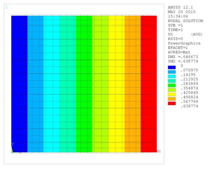 | Figure 5. Displacement contour Ux for evaluation of longitudinal properties E1 and v12 |
The values of Young’s modulus (E1) obtain from the ANSYS displacement contour results for varying fiber volume fractions (Vf) are plotted in a graph (Figure 6) with the results of analytical methods such as rule of mixture, Halpin-Tsai, Nielsen and Chamis.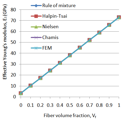 | Figure 6. Young’s modulus E1 with fiber volume fraction Vf |
The graph clearly shows that the E1 increases linearly with varying fiber volume fraction Vf. The effective Young’s modulus (E1) values obtained from FEM analysis (ANSYS), Rule of mixture, Halpin-Tsai, Nielsen and Chamis method gives very good predictions. Note that the Halpin-Tsai and Nielsen equation for longitudinal Young’s modulus share the same formulation as that of rule of mixture. In composite system less stiff polymer matrix is replaced by stiffer fiber material. Thus it is obvious that as fiber percentage increases the composite become stiffer and gives higher Young's modulus. This behavior is also demonstrated by FEM.
4.2. Evaluation of Major Poisson’s Ratio (ν12)
The values of Poisson’s ratio (v12) obtain from the ANSYS displacement contour results for varying fiber volume fractions (Vf) are plotted in a graph (Figure 7) with analytical methods such as Rule of mixture, Halpin-Tsai and Chamis. The effective Poisson’s ratio decreases linearly with increases in fiber volume fraction. Computational (FEM) results perfectly match the values of all the analytical methods. As the stiffness increases deformation of the composite decreases. Thus, effective major Poisson's ratio shows declining trend.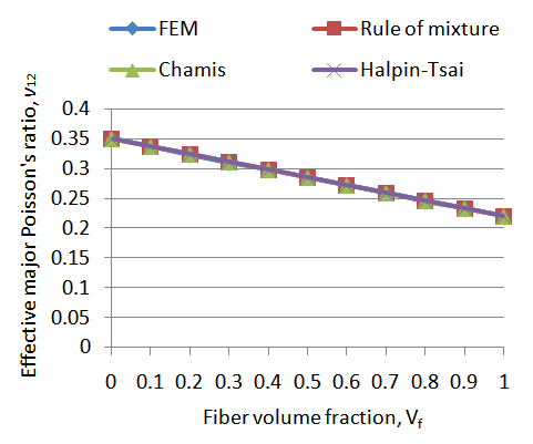 | Figure 7. Poisson’s ratio v12 with fiber volume fraction Vf. |
4.3. Evaluation of Transverse Young’s Modulus (E2)
The values of Young’s modulus (E2) obtain from the ANSYS displacement contour results for varying fiber volume fractions (Vf) are plotted in a graph (Figure 8) with other methods such as Rule of mixture, Halpin-Tsai, Nielsen and Chamis. A non-linear relationship is observed between fiber volume fraction and modulus. The value of Young’s modulus E2 increases as fiber volume fraction increases. The Halpin-Tsai and Chamis methods overestimate the FEM results, while Rule of mixture results matches well with the FEM results. Nielsen method shows severe deviation at 80% and 90% fiber volume predictions. However with in practical range (30-70%) of fiber content Nielsen method also shows good agreeing results.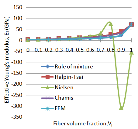 | Figure 8. Young’s modulus E2 with fiber volume fraction Vf |
The fiber percentage has shown very less effect on the effective Young's modulus E2 up to 80%. The fibers are strongest in the direction of loading and it will contribute to the loading capacity of fiber. However in the transverse direction change in the fiber volume will not show any benefit. The load applied in the direction of fiber gives more effective Young's modulus.
4.4. Evaluation of Minor Poisson’s Ratio (ν21)
Predicted values of effective minor Poisson’s ratio v21 with varying fiber volume fraction are shown in Figure 9. It is observed that the graph is non-linear, Poisson’s ratio decreases till it reaches its minimum value and then gradually increases as the fiber volume fraction increases. The minimum value of Poisson’s ratio (v21) in the FEM method is 0.054 at 0.5 and 0.6 fiber volume fraction. The variation of results between FEM and Rule of mixture method is very small. The percentage of the fiber volume fraction from (10-90%) has shown less influence in the effective minor Poisson's ratio. In the particular range of the fiber volume (30-70%), the fiber percentage has not shown any considerable influence on the effective minor Poisson's ratio.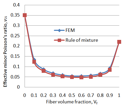 | Figure 9. Poisson’s ratio v21 with fiber volume fraction Vf |
4.5. Evaluation of Shear Modulus (G12)
ANSYS displacement contours results for the 0.4 fiber volume fraction along X direction (Ux-displacement) to evaluate shear modulus is shown in Figure 10. The values of effective shear modulus (G12) obtain from the ANSYS displacement contour results for varying fiber volume fractions (Vf) are plotted in a graph (Figure 11) with analytical methods such as Rule of mixture, Halpin-Tsai and Chamis.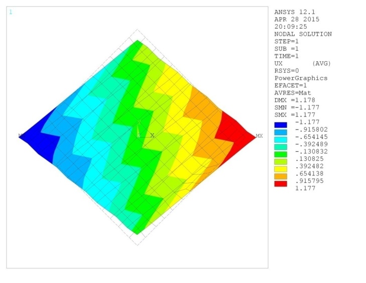 | Figure 10. Displacement contour Ux to evaluation of shear modulus G12 |
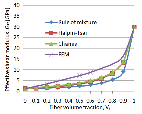 | Figure 11. Shear modulus G12 with fiber volume fraction Vf |
Graph shows non-linear nature between effective shear modulus and fiber volume fraction. Effective shear modulus G12 gradually increases with varying fiber volume fraction. It is shown that the Rule of mixture, Halpin-Tsai and Chamis overestimate FEM method. In the practical range of (30-70%) fiber volume fraction the shear modulus value is doubled. As the fiber percentage increases the shear modulus also increases. Thus the fiber will also contribute to the better performance of composites under shear loading. However greater significance is obtained only at higher fiber volume fractions. FEM results are higher compared to the Halpin-Tsai results at 40% fiber volume by 117%. The large difference in the moduli values between epoxy matrix and glass fiber could be the reason for such large variation in the values of Shear modulus G12 between FEM and analytical methods.
5. Conclusions
The present work includes details of extensive study on epoxy/glass composites, to determine the Effective Elastic Moduli using FEM methodology. Following are the important observations from the study.1. FEM results of effective Young’s moulus E1 and E2 shows good agreement with predicted values of analytical methods like rule of mixture, Halpin-Tsai, Nielsen and Chamis method. The longitudinal Young’s modulus E1 increases linearly where as transverse Young’s modulus E2 shows gradual (non-linear) increase as the fiber volume fraction increases from 0% to 100%.2. Effective Poisson’s ratio v12 and v21 also shows close agreement with predicted values of analytical methods. The major Poisson’s ratio v12 increases linearly where as minor Young’s modulus v21 decreases till it reaches its minimum value and then increases as the fiber volume fraction increases. The maximum deviation of v21 is 13% at 60% fiber volume fractions. 3. Effective shear modulus G12 gradually increases with varying fiber volume fraction. Results of FEM overestimate the shear modulus compared to other analytical methods with maximum deviation of 117% at fiber volume 40%.From the above observations, we can conclude that the elastic Young's modulus and Poisson's ratio determined using finite element method gives good comparison with analytical methods for varying percentage fiber volume in epoxy/glass composite system. However for shear modulus finite element method gives higher results compared to analytical methods.
References
| [1] | R.M. Jones, Mechanics of Composite Materials, McGraw-Hill, New York, 2nd ed., 1975. |
| [2] | K. K. Chawla, Composite Materials - Science and Engineering, Springer-Verlag, New York, 3rd ed., 2012. |
| [3] | Y.Y. You, J.J. Kim, S.J. Kim and Y.H. Park, 2015, Methods to enhance the guaranteed tensile strength of GFRP rebar to 900 MPa with general fiber volume fraction, Construction and Building Materials, 75, 54-62. |
| [4] | A. Patnaik, P. Kumar, S. Biswas and M. Kumar, 2012, Investigation on micro- mechanical and thermal characteristic of glass fiber reinforced epoxy based binary composite structure using finite element method, Computational Materials Science, 62, 142-151. |
| [5] | E. M. Jensen, D. A. Leonhardt and R. S. Fertig III, 2015, Effects of thickness and fiber volume fraction variation on strain field inhomogeneity, Composites Part A: Applied Science and Manufacturing, 69, 178-185. |
| [6] | A.J.M. Jasso, J.E. Goodsell, A.J. Ritchey, R. B. Pipes and M. Koslowski, 2011, A parametric study of fiber volume fraction distribution on the failure initiation location in open hole off-axis tensile specimen, Composites Science and Technology, 71(16), 1819-1825. |
| [7] | Y. Pan, L. Iorga and A. A. Pelegri, 2008, Analysis of 3D random chopped fiber reinforced composites using FEM and random sequential adsorption, Computational Material Science, 43(3), 450-461. |
| [8] | J. N. Reddy, An Introduction to the Finite Element Method, McGraw-Hill, New York, 3rd ed., 2005. |
| [9] | H.Z. Shan and T.W. Chou, 1995, Transverse elastic moduli of unidirectional fiber composites with fiber/matrix interfacial debonding, Composites Science and Technology, 53, 383-391. |
| [10] | S.I. Krishnamachari and L.J Broutman, Applied Stress Analysis of Plastics: A Mechanical Engineering Approach, Springer, 1st ed., 1993. |
| [11] | C.C. Chamis, 1989, Mechanics of Composite Materials: Past, Present, and Future, Journal of Composites Research and Technology, 11(1), 1989, 3–14. |
 Abstract
 Reference
 Full-Text PDF
 Full-text HTML