1. Introduction

Wind load and wind-resistance performance of wind-sensitive structures such as high-rise buildings, long-span bridges and large-roof structures are the great concerns of structural engineers. Because the structures are immersed in an Atmospheric Boundary Layer (ABL), appropriate modeling of an ABL is a premise of the procedure in estimating the dynamic interaction between the wind and structure. Modeling of an ABL usually involves the modeling of statistical features of the flow such as mean velocity, turbulence intensity, power spectrum and so on, but sometimes also requires the reproduction of the time series of wind speed when transient features of the wind are the study subject. This paper introduces the mathematical, wind tunnel and CFD approaches adopted to model the ABL flow in the structural wind engineering filed. The necessity of considering the organized turbulence structure of the ABL is emphasized. In addition, CFD simulations of the ABL over hilly terrain and sea surface are introduced as examples of the CFD approach.

2. Mathematical Methods

A fast Fourier transform (FFT) based mathematical method is often employed to transform signals between time (or spatial) domain and frequency domain, which has many applications in physics and engineering [Bracewell R.N. (1986), Brigham E.O. (1988)]. One of the most important parts of the mathematical simulation methodology is the generation of the stochastic processes, fields and waves involved in the problem. The generated sample functions must accurately describe the probabilistic characteristics of the corresponding stochastic processes, fields or waves that may be either stationary or non-stationary, homogeneous or non-homogeneous, one-dimensional or multi-dimensional, univariate or multi-variate, Gaussian or non-Gaussian [Shinozuka and Deodatis (1996)]. Initially, the mathematical simulation techniques focused on the generation of one-dimensional and univariate processes. The simulation of processes with more than a single dimension or a single component was first addressed by Borgman [1969] and Shinozuka [1970, 1972], and Shinozuka and Jan [1972]. Traditionally, the method based on the summation of trigonometric series with random phase angles has been the most popular, perhaps due to its simplicity. The multivariate processes are generated by implementing a stochastic decomposition scheme that exploits the concept of decomposing a set of correlated processes into a number of component processes. When the cross-spectral density matrix of an n-variate process is specified, its component processes can be simulated as the sum of cosine functions with random frequencies and random phase angles. Meanwhile, simulation of multivariate processes based on digital filtering was accomplished by first simulating a family of uncorrelated processes and subsequently imposing the appropriate correlation structure by a transformation [Li and Kareem 1993]. More developments in digital filtering techniques include state space modeling, autoregressive (AR), moving average (MA), and the combination autoregressive and moving averages (ARMA) models [Kareem 1987, Reed and Scanlan 1984, Li and Kareem 1993]. In addition, the wavelet transform, Hilbert transform and POD analysis have been incorporated into the mathematical approaches, which make the simulation of evolutionary characteristics of transient winds possible [Kitagawa and Nomura 2003, Wang 2006].

Although the above techniques vary in their applicability, complexity, computer storage requirement, and computing time, many simulated data show excellent agreement with the specified wind features, including the target spectral characteristics of the wind that makes the mathematical method very suitable to wind engineering application. The mathematical technique has immediate applications to the simulation of real-time processes, e.g., simulate the evolutionary characteristics of transient winds in order to explore the non-stationary thunderstorm wind loading on structures [Wang et al. 2013]. Meanwhile, the time-dependent velocity fluctuations modeled by mathematical approach are often utilized as the inlet flow boundary condition for the CFD approach. On the other hand, the movement of wind flow in the ABL is determined by the governing equations of the fluids, so the atmospheric turbulence is not a pure random process. It contains organized turbulence structures as other turbulent boundary layers. However, with more wind speed features considered in the process of mathematical simulation, we may expect that the simulated flow field approaches to the real one and is suitable to wind engineering application.

3. Wind Tunnel Modeling

The model test in a wind tunnel is considered the most reliable approach to study the wind effects on structures. The current wind load codes/standards are formulated under the premise that wind loads on structures are simulated in wind tunnels. The pioneer researchers in the wind engineering field such as Danvenport, Cermark, Cook and others had established the experimental technique related to the boundary layer wind tunnel test while creating the framework of wind resistant design of structures [Daveport and Isyumov 1967, Cermak and Cochran 1992]. In short, wind tunnel simulation of ABL is a well established practice, and the boundary layer wind tunnel has become a necessary tool for wind resistance design. In order to investigate the wind effects on structures realistically, the model tests should be conducted in wind tunnel flows with characteristics similar to those of natural wind. The natural atmospheric boundary layer over a variety of ground conditions are categorized into a limited number of terrain categories, which can be modeled in the boundary layer wind tunnels by different combinations of passive devices including spires, barriers and roughness blocks. Based on the assumption that velocity fluctuations can be adequately modeled by stationary mean and turbulent flow properties, attempts to simulate an atmospheric flow in a wind tunnel have so far been confined to the reproduction of the statistical characteristics, including power spectrum, vertical profiles of mean velocity and turbulence intensity and sometimes coherence.

Special devices are sometimes added into the wind tunnel to achieve a better modeling of a particular feature of the atmospheric turbulence, such as turbulence intensity [Teunissen 1975]. Makita developed a turbulence generator to model homogeneous flow field with high turbulence Reynolds number. Kobayashi [1994] and Nishi and Miyagi [1993] considered that the simulation of wind velocity history was of equal importance with the reproduction of the statistics. If the “raw” wind velocity history can be reproduced and the wind effects on structures are investigated in it, the obtained results would be more convincible. Fig.1 compares the time histories of the target and reproduced wind speeds in a multiple-fan wind tunnel [Nishi et al. 1999]. Recently a huge wind storm facility was built at the Insurance Center for Building Safety Research with a capacity to generate Category 3 winds (>130 mph) on a 220 sq m two-story building [Smith 2009].

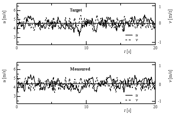Figure 1. Comparison of the target and modeled wind speeds

4. CFD Approach

Computational Fluid Dynamics (CFD) is basically a numerical approach to simulating or predicting phenomena and quantities of a flow by solving the equations of motion of the fluid at a discrete set of points. It has wide applications in flow-related engineering fields including aeronautical, mechanical and civil/architectural fields, although the difficulties in applying it to particular problems in these fields are different. The structural CWE usually involves the combination of problems of bluff body aerodynamics, inflow turbulence, wake turbulence, grid generation and high Reynolds number (up to the order of 10⁷ to 10⁸). All these problems require special attention in numerical simulation.

Many fundamental CFD studies have been conducted to simulate the turbulent channel or half-channel flow, in order to check the performance of numerical method or turbulence model as well as in order to investigate the characteristics of the boundary layer over smooth or rough plates. CFD has been shown to be very powerful in predicting wind field over kinds of terrain categories. In this paper, two examples of CFD simulation of turbulent boundary layers over hilly terrain and sea surface are provided.

ABL over hilly terrain

Turbulent flow over hilly terrain involves complicated flow phenomena such as spatial development, stable or unstable, i.e., intermittent, separation and reattachment according to the hill slope, and downstream recovery of the turbulent boundary layer. Thus, any disturbance that may influence the behavior of the separated shear layer and its interaction with the ground would change the global and local turbulent structure and thus influence the wind characteristics around hilly terrain. The slope of hilly terrain and the surroundings, especially upstream roughness conditions, are two important factors in determining the dynamic behavior of the turbulent boundary layer over a hilly terrain. With the increased concern about wind energy and wind loading problems in hilly terrains, many investigations have studied the turbulent boundary layer flow over an isolated hill, which is usually a start point in research on flow over complex terrain. In this study two representative hill shapes were considered, i.e., a steep one with stable separation and a low one without stable separation, as well as two representative upstream roughness conditions, i.e., a smooth one and a rough one corresponding to two kinds of velocity profile of the incoming flow.

Generation of inflow turbulence and modeling the effects of roughness blocks play important roles in simulating the turbulent boundary layer over hills. Spatially developing turbulent boundary layers over smooth and rough plates were simulated to generate the inflow turbulence. The methods of Lund et al. (1998) and Nozawa and Tamura (2002) were applied for the smooth and rough surface conditions, respectively. The point of Lund’s method of generating inflow turbulence was to rescale the velocity field at a downstream station, and re-introduce it as a boundary condition at the inlet, to allow for the calculation of spatially developing boundary layer in conjunction with pseudo periodic boundary conditions applied in the stream wise direction. The method of Nozawa and Tamura (2002) is an extension of Lund’s method for rough wall conditions. Meanwhile, rectangular blocks were arranged on the ground/hill surface to simulate the rough condition. An immersed boundary method (IBM) proposed by Goldstein et al. (1993) was used to model the no-slip boundary condition at all surfaces of roughness elements by adding an external force term in the governing equations of fluids. Note that the no-slip boundary condition was not imposed directly at the surfaces of the roughness elements. The coupling of the external force and the time derivative acceleration term corresponded to a kind of oscillation system. Fig. 2 and Fig.3 illustrate the instantaneous flow field over a smooth steep hill and a rough low hill respectively.

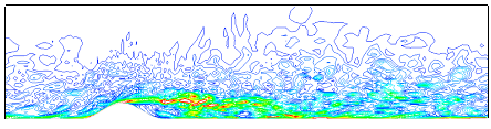Figure 2. Contours of the instantaneous vorticity magnitude over smooth steep hill

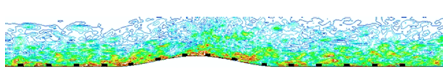Figure 3. Contours of the instantaneous vorticity magnitude over a rough low hill

ABL over sea surface

Wind load codes/specifications usually consider sea exposure as the smoothest condition of ground roughness, and specify a smallest power law index for the mean velocity profile at the coast. However, many field measurements have shown that sea surface wind stress, drag coefficient and aerodynamic roughness length are depended on the coupling effect of wind-wave interaction (e.g. Charnock 1955). Waves may perform as surface roughness in determining the boundary layers. Powell et al (2003) analyzed the wind velocity profiles over oceans measured by GPS sonde during tropical cyclones and reported reduced drag coefficient for high wind speeds in tropical cyclones. It means that the roughness length does not increase with the increase in wind speed at high wind speed. The sophisticated air flow field over waves is in great need of investigation as a guarantee of human offshore activities and facilities involved with oceans, such as oil and natural gas exploitation, long span sea bridges and offshore wind turbine farms that are sensitive to wind loads. Thus, study of the mean velocity profile and turbulence structure of atmospheric boundary layers over waves is an important and urgent issue to solve for wind engineers.

The air-sea interface is a complex system of interacting waves and atmospheric turbulence over a wide variety of spatial and temporal scales. The exchange of momentum and energy across the sea surface, for the most part, occurs on a molecular scale, involving both turbulent and laminar processes modified by wave breaking, surface tension, the structure of the wind boundary layer, and the ocean mixed layer, among other effects. Although the oceanographers and meteorologists have conducted many studies concentrating on sea surface wind stress, drag coefficient or its counterpart aerodynamic roughness length, the parameterizations of wind stress and wind profile still remain controversial, especially in high wind and very young sea conditions (Jones and Toba, 2001). Recently, Sullivan (2000, 2008) conducted a series of study on the flow over waves based on Couette-flow approximation. In the present study, Large-eddy simulation (LES) is performed to study the mean velocity profile and turbulence structure of fully developed Atmospheric Boundary Layers (ABL) over waves. The Reynolds number that is based on wavelength λ and bulk velocity of the air U_b is 10⁴. The water waves are idealized to be two-dimensional, periodic, non-evolving waves. Different wave steepness defined by a⁄λ(a: wave amplitude) and wave age defined by c⁄U_b (c: phase velocity of the wave) are considered. Furthermore, wave ages are categorized into three groups, i.e., wave moves upstream against wind, downstream with a speed lower or higher than wind, for which different characteristics of the mean velocity profiles and velocity fluctuation profiles are elaborated. This study is aimed to provide the information about wind characteristics off the coast during typhoons for wind engineering applications.

The dependence of the characteristics of atmospheric boundary layer over waves on both wave age and wave steepness is investigated systematically in this study. Three kinds of wave steepness are considered to study the effects of wave steepness, i.e., 0.025, 0.05 and 0.075, corresponding to small, medium and large wave amplitude. Another important parameter concerned in this study is the wave age c/U_b that describes the evolution state of wave. Wave ages are categorized into three groups, i.e., wave moves upstream against wind, downstream with a speed slower or faster than wind. Concretely, c/U_b =-0.5 (wave opposing wind), 0.5 (wave following wind) and 1.5 (wind following wave) are considered for 0.025 and 0.075, while more velocity combinations, i.e., c/U_b =-1.5, -1.0, -0.5, 0, 0.5, 0.75, 1.0, 1.5 and 2.0 are considered for 0.5 to elaborate the different characteristics of the mean velocity profiles and velocity fluctuation profiles over waves.

Fig.4 illustrates the mean velocity profiles at different wave ages at a/λ=0.05. β denotes wave age in Fig.4. The mean velocity profiles of the flow over a flat plate and a stationary wave are shown together as references. The mean velocity is averaged both in span-wise direction and in phase. The change of gradient height and power law index, and the change of roughness length and friction velocity with wave age are illustrated in Fig.5a and Fig.5b respectively.

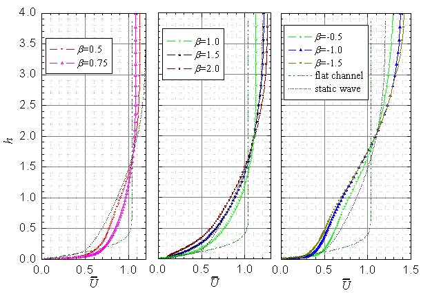Figure 4. Mean velocity profiles over waves at different wave ages

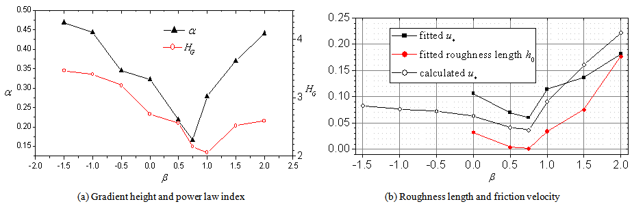Figure 5. Change of aerodynamic parameters associated to velocity profile

5. Conclusions

This paper introduces the improvements of mathematical, physical and CFD approaches utilized to model the Atmospheric Boundary Layer flow for structural wind engineering applications. CFD simulations of the ABL over hilly terrain and sea surface are introduced as examples of CFD approach. More detailed description and comparison of these methods will be presented at the conference.

ACKNOWLEDGEMENTS

This research was funded in part by Natural Science Foundation of China (NSFC) Grant number 51278366, and the 973 project of Ministry of Science and Technology.