B. S. Dhekale, P. K. Sahu, Vishwajith K. P., Md Noman, L. Narsimhaiah
Department of Agricultural Statistics, Bidhan Chandra Krishi Vishwvidyalaya, Mohanpur, Nadia, West Bengal
Correspondence to: B. S. Dhekale, Department of Agricultural Statistics, Bidhan Chandra Krishi Vishwvidyalaya, Mohanpur, Nadia, West Bengal.
| Email: |  |
Copyright © 2015 Scientific & Academic Publishing. All Rights Reserved.
Abstract
Murshidabad district of West Bengal is well known for agriculture potential with cropping intensity of more than 200%. About 70 % of total agricultural land yields 3 crops annually and the rest single crop. It is also marked with annual population growth rate of 4 % (Khatoon and Mondal, 2012). Irrigation in this area is almost wholly groundwater based. Various reports on ground water depletion concluded that Rarh area of this district shown continuous depletion in last three decades (Mohalla and Khatoon, 2013). This research aims at forecasting ground water fluctuations using time series analysis. Groundwater table data from each station under Murshidabad district was collected and analyzed station wise according to availability. The time series water table observations collected for four months January, May, August and November during the period from 2005 to 2013. Structural time series modeling technique was applied to model and foresee behavior of groundwater table in 2014. Data from 2005 to 2012 was used for analysis and 2013 data used for validation. Residuals of developed model for each station was tested for normality and randomness. Chi-square test used to test goodness of fit of model. On the basis of significance of parameters, residual analysis and goodness of fit, models were selected and used for forecasting purpose.
Keywords:
Groundwater, Murshidabad, Structural time series
Cite this paper: B. S. Dhekale, P. K. Sahu, Vishwajith K. P., Md Noman, L. Narsimhaiah, Structural Time Series Analysis towards Modeling and Forecasting of Ground Water Fluctuations in Murshidabad District of West Bengal, International Journal of Ecosystem, Vol. 5 No. 3A, 2015, pp. 117-126. doi: 10.5923/c.ije.201501.17.
1. Introduction
Groundwater is one of the most valuable natural resources and it has become a dependable source of water in all climatic regions of the world (Todd and Mays, 2005). In the developing countries, it is emerging as a poverty-alleviation tool owing to the fact that groundwater can be delivered directly to poor communities more cost effectively, promptly and easily than the surface water (IWMI, 2001). The shallow water table depths have significant impacts on crop growth, vegetation development and contaminant transport. Unfortunately, the dwindling of groundwater levels and aquifer depletion due to over-exploitation together with growing pollution of groundwater are threatening the sustainability of water supply and ecosystems. Furthermore, depletion of groundwater supplies, conflicts between groundwater users and surface water users, potential for ground water contamination are concerns that will become increasingly important as further aquifer development takes place in any basin. The consequences of aquifer depletion can lead to local water rationing, excessive reductions in yields, wells going dry or producing erratic ground water quality changes, changes in flow patterns of ground water resulting for example in the inflow of poorer quality water. So a constant monitoring of the groundwater levels is extremely important.India is a country where more emphasis has been given to boost up agriculture production. From the last few decades gradual depletion of groundwater supplies as a consequence of continued population growth and initiation of Boro cultivation over the Gangetic moribund delta has now been considered as an emerging problem. Murshidabad district is well known for agriculture potential with crop rating of more than 200%. About 70 % of total agricultural land yields 3 crops annually and the rest single crop (Khatoon and Mondal, 2012). During 2006-07 the district registered the largest gross cropped area (976 thousand hectares) in the state. The district also witnessed the second highest cropping intensity (245%) in the state during the period. The district recorded increase in area under total rice and Boro rice. During 2006-07 the district recorded second largest area under fruits (24.0 thousand) in the state. During the same period it has been observed that the district ranked 1st in terms of area under vegetables cultivation (81.2 thousand) in the state (Mohalla and Khatoon, 2013). It is also marked with annual population growth rate of 4 % (Khatoon and Mondal, 2012). Irrigation in this area is almost wholly groundwater based. Increasing population, agricultural use and urbanization extends heavy pressure on ground water table. Ground water table in the Rarh area of this district is showing continuous depletion in last three decades (Mohalla and Khatoon, 2013). In this regard monitoring, analyzing of groundwater level is necessary for assessing its quantity for planning purpose.Groundwater modeling has emerged as a powerful tool to help water managers to optimize groundwater use and to protect this vital resource. Various scientist forecasted groundwater fluctuations using various statistical techniques like Artificial Neural Network (ANN), Seasonal ARIMA modeling under different situations (Sahoo and Jha, 2013, Adhikari et al., 2012). Here in this paper we used structural time series modeling technique to model and forecast ground water fluctuations in Murshidabad district of West Bengal.
2. Material and Methods
To study the ground water fluctuation in Murshidabad district data on ground water table was collected from ground water information system for the period 2002 to 2013 for 29 stations of Murshidabad district. Data were available for the month of January, May, August and November. Descriptive statistics are used to describe the basic features of the data in any study. Descriptive statistics provide simple summaries about the sample data. The most widely used descriptive measure of central tendency and dispersions like arithmetic mean, range, standard deviation Skewness and kurtosis are used to explain each series.Structural time series technique was used for modeling and forecasting purpose. A “Structural time series model” has got four components, like trend, cyclical fluctuations, seasonal variations and irregular component. If additive model is assumed, it took the form: | (1) |
Where Yt = Observed time series at time t, Tt = Trend, Ct = Cyclical, St = Seasonal,  = irregular component. As mentioned above a “Structural time series model” is obtained by using various time series components, like trend, cyclical fluctuations, seasonal variation and irregular term i.e.,
 | (2) |
All the four components are stochastic and disturbances driving them are mutually uncorrelated. It is not necessary that every time series model should include all the above mentioned components. Generally, the annual data are devoid of seasonal components, unless or otherwise, seasonal data are provided for many years.Local level model (LLM):State space form of univariate time series models consist of transition equation  and a measurement equation
  In which
  is an m x 1 state vector,
  is an w x 1 fixed vector,
  is a fixed matrix of order and
  and
and  and
and  are, respectively, a scalar disturbance term and an
  vector of disturbances which are distributed independently of each other. It is assumed that
  is white noise with mean zero and variance,
  and
and  is multivariate white noise with mean vector zero and covariance matrix Q. In the models considered here,
  and
and  will also be assumed to be normally distributed.Kalman filter:Kalman filter, a smoothing algorithm is used for obtaining best estimate of the state at any given point within sample. It is a set of mathematical equations that provides an efficient computational solution of least square method. It is a recursive procedure for computing optimal estimator of the state at particular time, based on information available till that time (Meinhold and Singpurwalla, 1983). Hyper parameters:Prediction and smoothing is carried out once the parameters governing the stochastic movements of the state variables have been estimated. Estimation of these parameters, known as “hyper-parameters”, based on Kalman filter.Prediction error decomposition:The likelihood function can be expressed in terms of one-step-ahead prediction errors, and these prediction error emerge as a by-product of the filter (Shumway and stoffer, 2000).If cyclical and seasonal component are absent then, Eq. (1) reduces to
 | (3) |
Then trend component  becomes a permanent component called as “level”. This model assumed to vary according to random walk, i.e.
 | (4) |
LLM is formed from equation (3) and (4) together. Theses equations are in state space form. Level  can be estimated and then using weighted average, forecast values are calculated from data points. Sample mean is best forecast and last observation will be forecast if
  , and level is steady when
  . Level of time series varies over the time depending on signal to noise ratio
 . Estimation of
  , conditional on
  and
and  is done recursively using Kalman filter and smoother (Harvey, 1996). Unknown parameters
  and
and  are treated as hyper parameters. Prediction error decomposition is used to evaluate the likelihood function by Kalman filtering. One step ahead prediction of level i.e. estimator of
  can be given
  once
once  and
and  known viz.,
 | (5) |
is evaluated recursively by Kalman filter. Prediction error variance 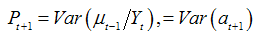 | (6) |
is also obtained recursively. Local liner trend model (LLTM): As described by Harvey (1996), LLTM is given by Eq. (3) along with the following two equations: | (7) |
 | (8) |
where
 and
and  . It may be mentioned that
  ,
,  and
and  are independent of one another. If
  equations (7) and (8) reduces to
  | (9) |
Which can equivalently be written as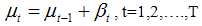 | (10) |
LLTM is in state space form with state vector 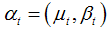 . Assuming that
  ,
,  and
and  are known updating and prediction are carried out using Kalman filter. Otherwise these can be estimated using maximum likelihood method for state space model (de Jong, 1988).Models are developed using structural time series technique and tested for significance of parameter. R square provides goodness of fit the model. Higher the value of R square model will be good. In addition to the above, two more reliability statistics viz., Root Mean Square Error (RMSE), Mean Absolute Error (MAE) and Mean Absolute Percentage Error (MAPE) are generally utilized to measure the adequacy of the fitted model and it can be computed as follows:
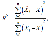
 where,
  are the value of the ith observation, mean and estimated value of the ith observation of the variable X.Residuals of developed model were tested for its randomness and normality using run test and Shapiro Wilks statistic respectively. Also
  square test is used to test the goodness of fit for observed and predicted values, non significance of test represents good fir. The models satisfying most of the criteria were selected for forecasting and then used for forecasting purpose.
3. Results and Discussion
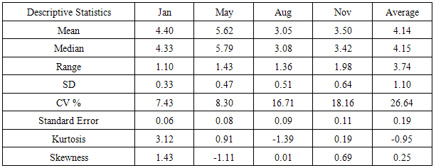
Results of descriptive statistics for Murshidabad district is given in table 1. It can be easily revealed that in May water table level is low 5.62 m as it is hottest month and in the month of August it is high 3.05 m. Value of standard deviation for November is higher (0.64) as compared to other months this may be due to reason of irregular behavior of receiving southwest monsoon and which causes more variation. Skewness for the month of May is negative indicating that water table depletion is more in lower water table values. Overall average ground water depth in Murshidabad is 4.14 m. Station wise descriptive i.e. mean and standard deviation were represented in fig.1 to fig.4. 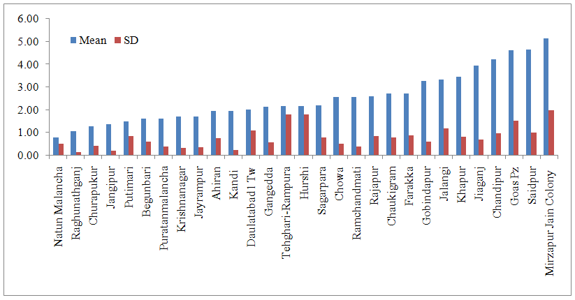 | Figure 1. Ground water table in the month of August in all stations in Murshidabad district |
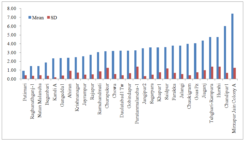 | Figure 2. Ground water table in the month of November in all stations in Murshidabad district |
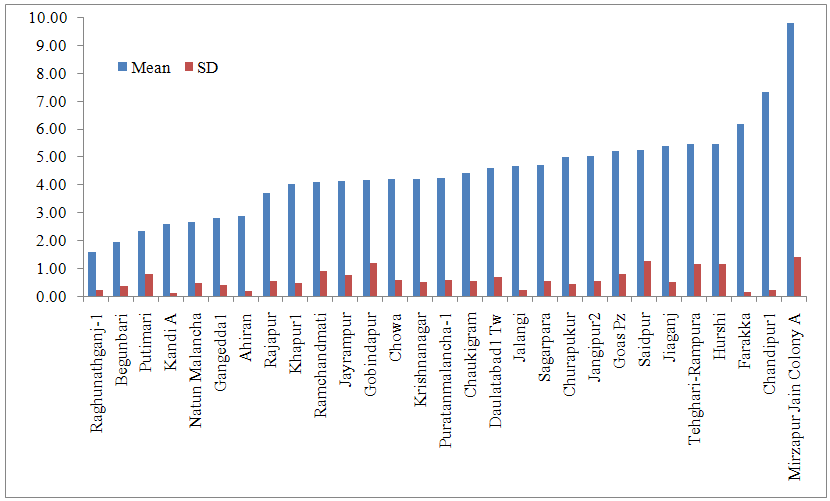 | Figure 3. Ground water table in the month of January in all stations in Murshidabad district |
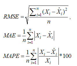
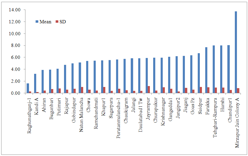 | Figure 4. Ground water table in the month of May in all stations in Murshidabad district |
Table 1. Per se performance ground water table of Murshidabad district
 |
| |
|
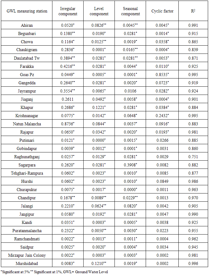
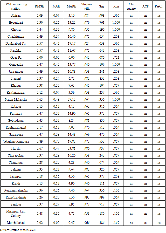
From fig 1 it is concluded that Natun Malancha station has highest water table of 0.79 m while lowest in Mirzapur jain colony of 5.13 m in August month. Teleghari-Rampura and Hurshi stations showed more variation. These regions showed fluctuating water table over the years. This may be due to reason that these regions receives varied rainfall.In November month overall Mirzapur Jain colony showed deep water table while Putimari showed shallow water table (Fig 2). Overall water table ranges in between 0.79 m to 7.80 m. Hurshi, Tehghari-Rampura, and Chandipur stations showed deep water table continuously. Variations in the depth of water table across the sites for the month of January have been presented in fig. 3. Raghunathganj showed shallow (1.60) water table and Mirzaur Jain colony showed deep (9.77) water table in January month. Standard deviation of both the stations was low as compared to mean hence it can be concluded that overall both stations showed consistent for shallow and deep water table. Thus compared to August and November, water table is declining during January month. This is mainly because Murshidabad district receives rainfall from the month of June to September, and after that water is pumped from tube wells and aquifer which affect water table positively. Among the four month of recording water table depth, May month is hottest month and Mirzapur Jain Colony showed deepest water table (13.69 m) while Raghunathganj showed shallow water table (1.61 m). Evaporation in this month is more and Murshidabad district not receiving rainfall this month, hence this month water table is deepest. If we compare water table across the months, Hurshi station observed more variation in water table depth. Water table in August month was 2.0 m, November (4.87 m), January (5.47 m) and May (7.99 m). Even Gangedda station observed water table around depth of 2 m in month of August, November and January while in the month of May it was 6.80 over the period of study. Structural time series technique was used, modeled and validated for all stations. Results of parameter estimates of structural time series models for each station are represented in table 2. Structural time series composed of cycle, trend, seasonal and irregularity. In cyclic component damping factor represents oscillating movement of a data. The damping factor for all sites was 0.90 i.e. equal to 1 which means every year cycle repeats and Period of cycle means time taken to go through its complete sequence of values. Period for analysis is constant for all sites and was 4 which means every four points cycle repeats. For all the stations, R square ranges between 0.84 and 0.99, residuals were normal and random (Table 2), ACF & PACF for residuals and also  square test (Table 3) were non-significant all together represents the correctness of fitted model. For Murshidabad district RMSE, MAE and MAPE values were 0.02, 0.02 and 0.47 respectively. These models are also validated for 2013 data and found that observed and predicted values are similar for all stations (Table 4).
Table 2. Model development in structural time series technique in Murshidabad district
 |
| |
|
Table 3. Residual analysis of structural time series modeling of groundwater table in Murshidabad district
 |
| |
|
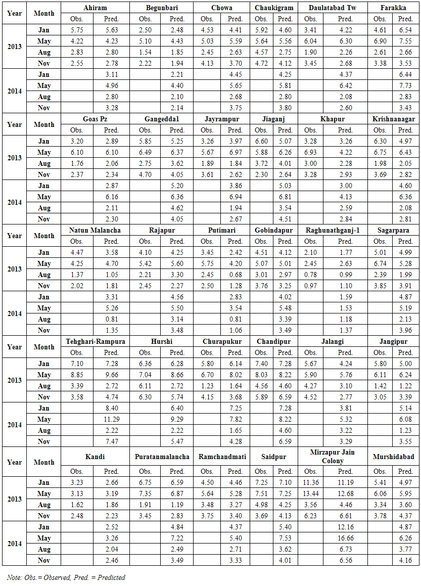 | Table 4. Observed and Predicted values of ground water table in Murshidabad district |
As parameters of models are significant and residuals are normal and random, forecasting of water table using structural time series modeling is done and presented in table 4. Fitting of structural time series model and forecasting for Murshidabad district is presented in fig. 5. 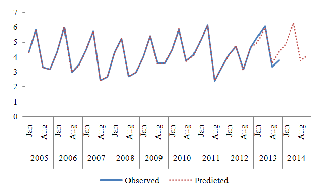 | Figure 5. Forecasting of ground water table for 2014 of Murshidabad district |
4. Conclusions
Study of ground water depth clearly indicates that there are differences among the sites of measurements as well among the season. Maximum variability among the sites in a particular season is found during the month of November followed by August as depicted by the CV value for the respective seasons. This clearly reflects that ground water recharge is different for different sites within a season also. Through structural time series modeling effectively model the water depth during different seasons. The method may not yield equally efficient forecast values, as future Hurshi and Chaukigrama during the month of May, Tehghari-Rampura, Hurshi Putimari, Puratan Manchala and Mirzapur Jain Colony during August. Thus this the modeling and forecasting should be applied with utmost care.
References
| [1] | Adhikari S. K., Rahiman M. and Das Gupta A. 2012, A Stochastic modeling technique for predicting groundwater table fluctuations with Time series analysis. International Journal of Agricultural Sciences and Engineering Research, 1(2), 237-249. |
| [2] | De Jong, P. 1988. The likelihood for a state space model. Biometrika, 75, 165-69. |
| [3] | Harvey, A.C. 1996. Forecasting, Structural Time-Series Models and the Kalman Filter. Cambridge Univ. Press, U.K. |
| [4] | IWMI. 2001. The strategic plan for IWMI 2000–2005. International Water Management Institute (IWMI), Colombo, pp 28. |
| [5] | Khatoon, N. and Mondal, S. 2012. Intensive irrigation practices and groundwater depletion in seven selected blocks in the Rarh (west of the Bhagirathi) in Murshidabad West Bengal. Indian Streams Research Journal, 6(2), 1-9. |
| [6] | Meinhol, R.J. and Singpurwalla, N.D., (1983). Understanding Kalman filter. Amer. Statistician, 37, 123-127 |
| [7] | Mollah, S. and Khatoon N. 2013. Water Scarcity in Agricultural Sector in Murshidabad, West Bengal. Global Research Analysis. 2(3), 161-163. |
| [8] | Sahoo, S. and Jha, M. K. 2013.Application of hybrid neural network in modeling water table fluctuations, Journal of Ground Water Reseach, 2 (1), pp 8-19 |
| [9] | Shumway, R.H. and Stoffer, D.S., (2000). Time series analysis and its applications. Springer Verlag, New York. |
| [10] | Todd, D. K. and Mays, L.W. (2005) Groundwater hydrology, 3rd edn. Wiley, Hoboken |
 Abstract
 Reference
 Full-Text PDF
 Full-text HTML