Soumik Ray, Banjul Bhattacharyya
Dept. of Agricultural Statistics, Bidhan Chandra Krishi Viswavidyalaya, Mohanpur, West Bengal
Correspondence to: Soumik Ray, Dept. of Agricultural Statistics, Bidhan Chandra Krishi Viswavidyalaya, Mohanpur, West Bengal.
| Email: |  |
Copyright © 2015 Scientific & Academic Publishing. All Rights Reserved.
Abstract
Irrigation is the artificial application of water to the land or soil. It is used to assist in the growing of agricultural crops, maintenance of landscapes, and revegetation of disturbed soils in dry areas and during periods of inadequate rainfall. Irrigation has been a central feature of agriculture for over 5000 years, and was the basis of the economy and society of numerous societies, ranging from Asia to Arizona. In our country the sources of irrigation water can be groundwater extracted from springs or by using tanks, wells, canals, river and other artificial projects for the purpose of cultivation and agricultural activities. India has an irrigation potential of 139.89 million hectares, out of which a minimal 108.2 million hectares (77.35%) of the total land that can be irrigated has been utilized. Currently, about 30% of the net cultivated area has benefited from the irrigation projects that have been implemented. A sum of  16,590 crore has been spent of irrigation development up to the 7th Five-Year plans of India. The 10th and 11th Five Year Plan have proposed to invest a sum of
  1,03,315 crore and 2,10,326 crore on irrigation and flood control in India. So it has become very much required to re-examine the different source of irrigation scenario and related policy issues in the present context. The present dissertation works are designed in demographic pattern and future projection of irrigation sources in India.
Keywords:
ARIMA, ACF, PACF, AIC, SBC, MAPE
Cite this paper: Soumik Ray, Banjul Bhattacharyya, Availability in Different Source of Irrigation in India: A Statistical Approach, International Journal of Ecosystem, Vol. 5 No. 3A, 2015, pp. 109-116. doi: 10.5923/c.ije.201501.16.
1. Introduction
Irrigation is the artificial application of water for the cultivation of crops, trees, grasses and so on. For a typical Indian farmer, looking up to the skies to see whether the rain gods will favour him this time, irrigation means a wide range of interventions at the farm level, ranging from a couple of support watering(s) (or ‘life saving’ watering) during the kharif (monsoon) season from a small check dam/ pond/tank/dry well to assured year-round water supply from canals or tube wells to farmers cultivating three crops a year. The method of application has also evolved, from traditional gravity flow and farm flooding to micro-irrigation where water is applied close to the root zone of the plant. Indian farmers gain access to irrigation from two sources—surface water (that is, water from surface flows or water storage reservoirs) and groundwater (that is, water extracted by pumps from the groundwater aquifers through wells, tube wells and so on). Surface irrigation is largely provided through large and small dams and canal networks, run-off from river lift irrigation schemes and small tanks and ponds. Canal networks are largely gravity-fed while lift irrigation schemes require electrical power. Groundwater irrigation is accessed by dug wells, bore wells, tube wells and is powered by electric pumps or diesel engines. To meet the growing needs of irrigation, the government and farmers have largely focused on a supply side approach rather than improve the efficiency of existing irrigation systems. India has an irrigation potential of 139.89 million hectares, out of which a minimal 108.2 million hectares (77.35%) of the total land that can be irrigated has been utilized. Currently, about 30% of the net cultivated area has benefited from the irrigation projects that have been implemented. A sum of  16,590 crore has been spent of irrigation development up to the 7th Five-Year plans of India. The 10th and 11th Five Year Plan have proposed to invest a sum of
  1,03,315 crore and 2,10,326 crore on irrigation and flood control in India. So it has become very much required to re-examine the different source of irrigation scenario and related policy issues in the present context. The present dissertation works are designed in demographic pattern and future projection of irrigation sources in India.
2. Objective
The so termed ‘minor’ irrigation is now the major source as groundwater provides 50 per cent of the gross area under irrigation (in fact recent data shows that in terms of net sown area, groundwater provides 60 per cent of the net irrigated area (Shah and Deb, 2004). Thus, groundwater is a critical element in filling the need gap for the rural farmers, as it has provided irrigation in areas where the public irrigation systems have not reached or where the service delivery has been poor. In the last two decades, 84 per cent of the addition to net irrigated area has come from groundwater.Analysis of trend and pattern of irrigation sources are the primary objective of this work. With this aim the following study are carried out.v To study the different sources of irrigation over the year.v To assess the condition of changing pattern of net and gross irrigated area in India.v To analyze the irrigation pattern over the year.
3. Material and Methodology
The data set is collected from census of India Report and Indiastat.com (http://www.indiastat.com/default.aspx). The data are taken for a period from 1950-2010.Trend analysis uses a technique called least squares to fit a trend line to a set of time series data and then project the line into the future for a forecast. Trend analysis is a special case of regression analysis where the dependent variable is the variable to be forecasted and the independent variable is time. While moving average model limits the forecast to one period in the future, trend analysis is a technique for making forecasts further than one period into the future.Linear model: The mean model described above would obviously be inappropriate here. Many persons, upon seeing this time series, would naturally think of fitting a simple linear trend model-i.e., a sloping line rather than horizontal line. The forecasting equation for the linear trend model is:
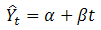 where t is the time index. The parameters alpha and beta (the "intercept" and "slope" of the trend line) are usually estimated via a simple regression in which Y is the dependent variable and the time index t is the independent variable.Exponential model: Exponential growth occurs when the growth rate of the value of a mathematical function is proportional to the function's current value. Exponential decay occurs in the same way when the growth rate is negative. In the case of a discrete domain of definition with equal intervals it is also called geometric growth or geometric decay (the function values form a geometric progression).The formula for exponential growth of a variable x at the (positive or negative) growth rate r, as time t goes on in discrete intervals (that is, at integer times 0, 1, 2, 3, ...), is
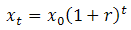 where x0 is the value of x at time 0.The ARIMA models:i) The Autoregressive (AR) Model: The Simplest form of the ARlMA model is called the autoregressive model. Let zt stand for the value of a stationary time series at time t, that is, a time series that has no trend, but fluctuates about a constant value referred to as the level of the series. (We deal with trends below.) By autoregressive, we assume that current zt values depend on past values from the same series. In symbols, at any t,
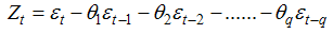
 Where C is the constant level, zt-1, zt-2,…..,zt-p are past series values (lags), the ’s are coefficients (similar to regression coefficients) to be estimated, and εtis a random variable with mean zero and constant variance. The εt‘s are assumed to be independent and represent random error. Some of the’s may be zero. If zt-p is the furthest lag with a nonzero coefficient, the AR model is said to be of order p, denoted AR (p).ii) The Moving Average (MA) Model: zt can also be modeled as a linear combination of white noise stochastic error terms. We call this type of model a moving average (MA) model. ifzt is considered as a weighted average of the uncorrelated εt 's , MA(q) moving average component of order q, which relates each zt value to the q residuals of the q previous z estimates may be expressed as
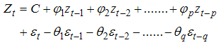
 iii) The ARMA Model: The AR and MA models for stationary series to account for both past values and past shocks may be combined. Such a model is called an ARMA (p, q) model with p order AR terms and q order MA terms. Thus an ARMA (p, q) model is written as
 Box-Jenkins method consists of the following steps:i) Identification: To identify the model of ARIMA (p,d,q) is based on the concepts of time-domain and frequency-domain analysis i.e. autocorrelation function (ACF), partial autocorrelation function (PACF) and spectral density function. The autocorrelation function (ACF) and partial ACF (PACF) are very important for the definition of the internal structure of the analyzed series. The ACF ρ(k) at lag k of the zt series is the linear correlation coefficient between zt and zt-k , calculated for k = 0, 1, 2...
 The PACF is defined as the linear correlation between zt and zt-k, controlling for possible effects of linear relationships among values at intermediate lags.Once the order of differencing has been diagnosed and the differenced univariate time series can be analyzed by the method of both time-domain and frequency-domain approach (Cressie, 1988).ii) Estimation: Having identified the appropriate p and q value the next stage is to estimate the parameter of the autoregressive and moving average terms included in the model. The appropriate p, d and q values of the model and their statistical significance can be judged by t-distribution. Akaike’s Information Criterion is adopted for model identification. The minimum value of AIC (Akaike’s Information Criterion), and SBC (Schwarz’s Bayesian Criterion) may be regarded as best fitted model. Standard computer package like SAS (Statistical Analysis System), SPSS etc. are available to finding the estimate of relevant parameters using iterative procedures. iii) Akaike information criterion (AIC): The Akaike information criterion is a measure of the relative goodness of fit of a statistical model. AIC values provide a means for model selection. AIC can tell nothing about how well a model fits the data in an absolute sense. In general case, the AIC is
  AIC = 2k - 2 ln (L)Where k is the number of parameters in the statistical model and L is the maximized value of the likelihood function for the estimated model.Schwarz Bayesian information criterion (SBC): In statistics, the Bayesian information criterion (BIC) or Schwarz criterion (also SBC, SBIC) is a criterion for model selection among a finite set of models. It is based, on the likelihood function, and it is closely related to Akaike information criterion (AIC).The formula for the BIC is -2∙ ln p(x│k) ≈ BIC = -2 ∙ln L+ k ln(n) iv) Diagnostic checking: Diagnostic checking consists of evaluating the adequacy of the estimated model. Considerable skill is required to choose the actual ARIMA (p,d,q) model so that the residuals estimated from this model are white noise. So the autocorrelations of the residuals are to be estimated for the diagnostic checking of the model. These are also judged by Ljung-Box statistic under null hypothesis that autocorrelation co-efficient is equal to zero. The Ljung-Box statistic, in case of large samples which follows a chi-square distribution with m degrees of freedom, is given by
 v) Forecast: The filtered data model is compared over forecast lead times 1 to 4 terms of mean absolute percentage error (MAPE) statistic. The relative measure of forecast accuracy is descripted by Koreisha & Fung (1999), and Pankratz (1983). The forecasts obtained by the fitted model are more reliable and forecast comparison can be carried out by the following statistic:
4. Result and Discussion
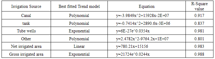
Different parametric trend models were fitted to the different irrigation sources i.e. tank, canal, tube wells, and other sources. The ARIMA model was fitted to the net irrigated area and gross irrigated area. The findings are discussed below.The best fitted trend models were find out for different sources of irrigation considered in this work for the period 1950-1951 to 2010-2011. Figure 1 represents the trend curve for different irrigation sources. The corresponding trend for irrigation sources and irrigated area are listed in table 1.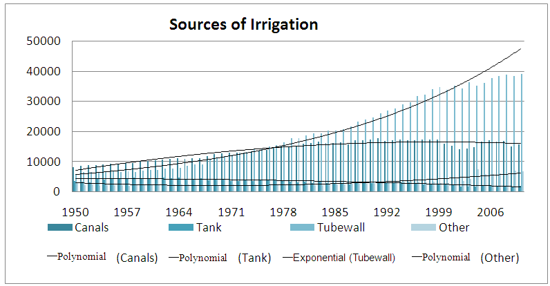 | Figure 1. Trend curve for sources of irrigation. (thousand hectare) |
Table 1. Best fitted trend for irrigation sources and irrigated area
 |
| |
|
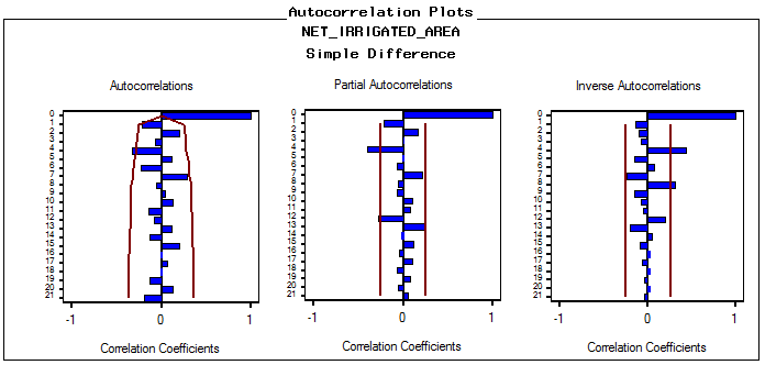
In ARIMA time series modeling the auto-correlations up to 21 lags were worked out. It is observed that both the univariate time series data are non-stationary in mean. The stationary series is the one whose values vary over time only around a constant mean and constant variance. There are several ways to ascertain this. The most common method is to check stationarity through examining the Correlogram graph or time plot of the data. Fig.2(a) and Fig.2(b) indicate the autocorrelation function and partial autocorrelation function of the historical observations of the net irrigated area and gross irrigated area in India. ACF remain close to 1.0 throughout, declining gradually. The PACF has the 1st spike significant and the others are non-significant. So the series have the ARIMA system as the other PACF spikes have a wave with positive and negative values. Difference is the produce for filtering the series. In both the cases the 1st difference series become stationary i.e. d was decided to be 1.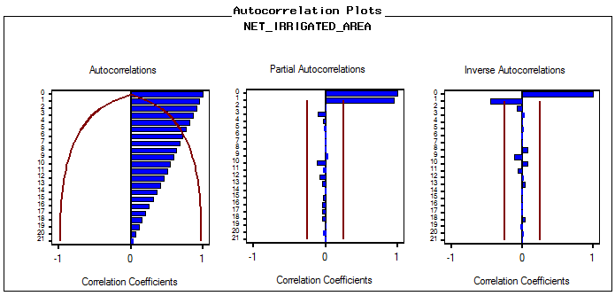 | Figure 2(a). Autocorrelation Plots of Time Series data for Net irrigated Area |
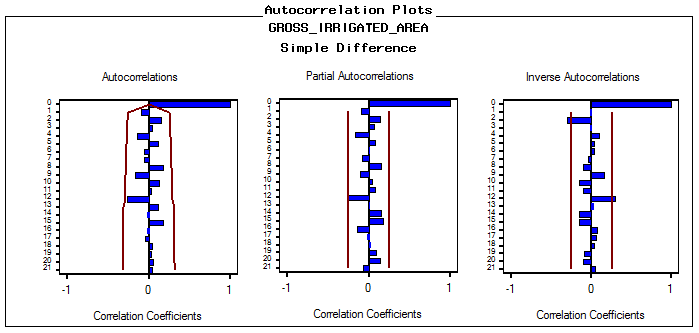
 | Figure 2(b). Autocorrelation Plots of Time Series data for Gross irrigated Area |
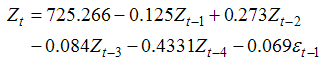
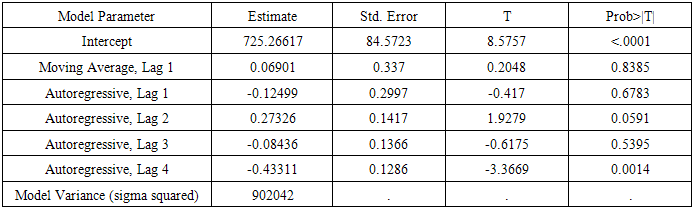
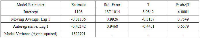
The next step is identification of the value of autoregressive process of order (p) and moving average process of order (q). The correlogram of Auto correlation function (ACF) and Partial Auto correlation function (PACF) of 1st difference series is utilized to identify ‘p’ and ‘q’. The correlogram for best fitted ARIMA model, represented in Fig. 3(a) and fig.3(b) for net irrigated and gross irrigated area respectively are accepted on the basis of Akaike information criterion (AIC), Schwarz Bayesian information criterion (SBC) and Mean Absolute Percentage Error (MAPE) and maximum R2 value which are given in table 2(a1) and table 2(b1). Table 2(a2) and table 2 (b2) shows the estimated parameters in this model. In case of net irrigated area ARIMA (4,1,1) model is found to be the best fitted one. And also for gross irrigated area ARIMA (1,1,1) model is the best one. The diagnostic checking of the model is concerned with the residual plots of ACF and PACF in both net and gross irrigated area in India. This is presented in Fig. 4(a) and 4(b). Fig.5 (a) and 5(b) shows the observed and expected data for the whole period with forecast values. In the basis of above results the model for estimation of net irrigated area may be represented mathematically as: 
 | Figure 3(a). Correlogram of ARIMA (4,1,1) model for net irrigated Area |
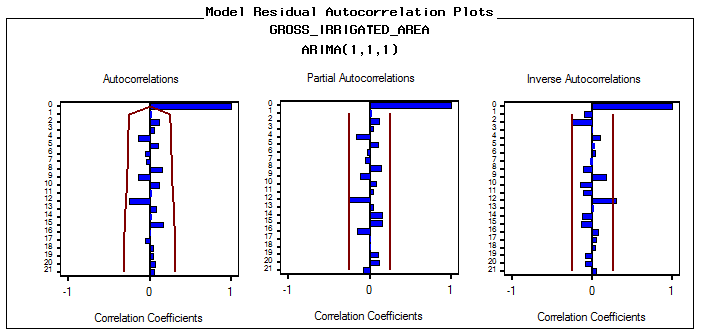
 | Figure 3(b). Correlogram of ARIMA (1,1,1) model for gross irrigated Area |
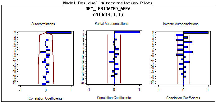 | Figure 4(a). Residual plot of ACF and PACF of net irrigated area |
 | Figure 4(b). Residual plot of ACF and PACF of gross irrigated area |
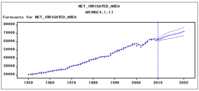 | Figure 5(a). Graphical representation of observed and fitted values along with Forecasts of net irrigated Area |
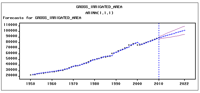 | Figure 5(b). Graphical representation of observed and fitted values along with Forecasts of gross irrigated Area |
Table 2(a1). Model Fit Statistics for net irrigated area
 |
| |
|
Table 2(a2). Parameter Estimates for net irrigated area
 |
| |
|
Table 2(b1). Model Fit Statistics for gross irrigated area
 |
| |
|
Table 2(b2). Parameter Estimates for gross irrigated area
 |
| |
|
And the model for estimation of gross irrigated area may be represented mathematically as:
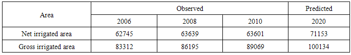
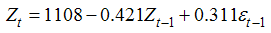 The ARIMA models developed in the present dissertation work finally are used to forecast the corresponding variables. Table 3 represents the observed and estimated values for net and gross irrigated area as obtained by respective ARIMA models.
Table 3. Forecast value for net and gross irrigated area. (thousand hectare)
 |
| |
|
5. Conclusions
The dissertation work intended to present a clear and comprehensive scenario of present status for different sources of irrigation and irrigated area in India in last three decades. The present work examined critically the secondary data collected from census of India Report and Indiastat.com (http://www.indiastat.com/default.aspx). The study period was considered from 1950-51 to 2010-11. Trend estimation and time series ARIMA modeling has been employed to develop appropriate models. Effort has also been taken to forecast the future trend of production along with the changing pattern of net and gross irrigated area in India.The analysis reveals the following observations:● The sources of irrigation i.e. canals, tanks, tube wells are shows the polynomial trend and exponential trend respectively.● Net irrigated and gross irrigated area in India both are in increasing trend. In net irrigated area the trend curve shows the linear trend whereas gross irrigated area are goes in exponential trend.● The univariate time series data for net and gross irrigated area are non-stationary in mean indicating existence of high autocorrelation.● All the univariate time series data considered in the study were treated separately. The partial autocorrelation function (PACF) has the 1st spike significant and the others are non-significant indicating the series possess the ARIMA system as the other PACF spikes have a wave with positive and negative values. So, differencing is the procedure for filtering the series.● For all the series under analysis suitable ARIMA models and estimated mathematical equations were developed and presented vividly in Result and Discussion.● We see that the supplies of water through tube wells are becoming the major source for irrigation. So we can concentrate about this source that can be utilized in irrigation for better crop production. Other sources are not increasing day by day. They are remaining approximately constant. We need to improve the irrigation sources for better irrigated area for better production.
References
| [1] | Agrawal R. and Jain R.C. (1996). “Forecast of sugarcane yield using eye estimate along with plant characters”. Biometrical Journal, 38(5):731-39 |
| [2] | Badmus M.A. and Ariyo O.S. (2011): “Forecasting Cultivated Areas and Production of Maizein Nigerian using ARIMA Model”. Asian Journal of Agricultural Sciences 3(3): 171-176. |
| [3] | E. Weiss (2000), Forecasting commodity prices using ARIMA, Technical Analysis of Stocks & Commodities, Vol. 18, No.1, pp.18-19, 2000. |
| [4] | http://www.iitk.ac.in/3inetwork/html/reports/IIR2007/07-Irrigation.pdf |
| [5] | http://en.wikipedia.org/wiki/Irrigation |
| [6] | http://www.indiastat.com/default.aspx |
| [7] | Iqbal N., Bakhshi K., Maqbool A. and Shohab A. Ahmad (2005). “Use of the ARIMA Model for Forecasting Wheat Area and Production in Pakistan”. Journal of Agriculture and Social Science; 1813–2235/2005/01–2–120–122. |
| [8] | Johansen, S. (1988). “Statistical Analysis of Co-integration Vectors”, Journal of Economic Dynamics and Control, (12):pp.231-254. |
| [9] | Ljung, G. and Box, G. (1978). "On a Measure of Lack of Fit in Time Series Models", Biometrika, 65,297-303. |
| [10] | Mandal B.N. (2005). Forecasting Sugarcane Production in India using ARIMA model, http://interstat.statjournals.net. |
| [11] | Melard, G. (1984). A fast algorithm for the exact likelihood of autoregressive-moving average models. Applied Statistics, 33:1, 104–119. |
| [12] | Ramasabramanian V. (2005). Time Series Analysis, http:// www.iasri.res.in/ebook. |
 Abstract
 Reference
 Full-Text PDF
 Full-text HTML