Balai Chandra Das1, Aznarul Islam2
1Assistant Professor in Geography, Krishnagar Govt. College, Nadia, West Bengal, India
2Assistant Professor in Geography, Barasat Govt. College, North24 Parganas, West Bengal, India
Correspondence to: Balai Chandra Das, Assistant Professor in Geography, Krishnagar Govt. College, Nadia, West Bengal, India.
| Email: |  |
Copyright © 2015 Scientific & Academic Publishing. All Rights Reserved.
Abstract
Attempt to measure channel asymmetry of cross-sectional area of a river was perhaps first taken by Knighton (1981). In the present paper it has been intended to devise some new perspectives on cross sectional asymmetry besides the Knighton’s three existing measures in this field. The theoretical and methodological observations have been validated with the help of an empirical study conducted on Nawapara Beel, an ox-bow lake in C.D. Block Krishnagar-II, Nadia, West Bengal, India. The work has been done using simple measures of trigonometry and mensuration.
Keywords:
Asymmetry-Area (Á), Bank-Full Width (w), Channel Centre Line (Lc), Channel Median Area Line (Lm)
Cite this paper: Balai Chandra Das, Aznarul Islam, Channel Asymmetry of an Ox-Bow Lake: A Different Perspective, International Journal of Ecosystem, Vol. 5 No. 3A, 2015, pp. 69-74. doi: 10.5923/c.ije.201501.10.
1. Introduction
Asymmetry is complementary to symmetry. They are two eternal essences of nature that keeps it dynamic. It is also true for the river channel cross-sectional form. About 90% channels are asymmetric (Leopold and Wolman, 1960). Cross-sectional forms are asymmetric even in straight channel (Majumder, 2011) with successive bars of alternating pitch (Einstein and Shen, 1964; Keller, 1972). To measure the degree of asymmetry of river channel cross-sectional form, Knighton (1981) has formulated three indices. Of these three indices, first one (A*) is very easyabd most scientific to measure the degree of asymmetry of channel cross-sectional form. However, second index (A1) and third index (A2), considered asymmetry in both directions i.e. horizontal and vertical (Knighton, 1981). In symmetrical channel, one half of the channel appears as laterally inversed virtual image of the other half (Gour and Gupta, 1998). So line on reflection plane may be considered as a center line of symmetry from which every point on object and corresponding points on virtual images appears to be at equal distance. Centre line (Knighton, 1981) of a cross-section, hence may be considered as a reference line of measurement of symmetry of the channel. But in case of vertical asymmetry, the reference line is not defined although difference between mean depth and maximum depth is considered to be used. With the words ‘increasing vertical asymmetry’ Knighton (1981), perhaps intended to show that, the maximum depth (dmax) is increasing while mean depth (d) is constant. But it seems that vertical asymmetry is not possible at all. Therefore what is to be considered in designing of an index of asymmetry of river channel cross-sections is simply ‘area’. As cross-sectional form itself is a two dimensional concept. So present paper has incorporated areal asymmetry as the principal point of consideration and used some simple statistical tools to the end.
2. Derivation of Asymmetry Measures
As stated by Knighton (1981), the existence and significance of asymmetry has been studied in allied fields, from the view points of both process action (Kranck, 1972; Clifton, 1976) and development (Sharp 1963; Tanne, r, 1967; Kennedy, 1976). Sharp (1963) defined asymmetry in wind ripple by length of shadow zone (Figure 1A). Tanner (1967) and Reineck and Wunderlich’s (1968) asymmetry index was the simple ratio of length of the horizontal projection of the stoss side to that of the lee side (Figure 1B). Contributions of Knighton (1981) in measure of channel asymmetry are useful tools to the understanding of channel geometry. However, asymmetry measures introduced in this paper is someway new and significant to the field.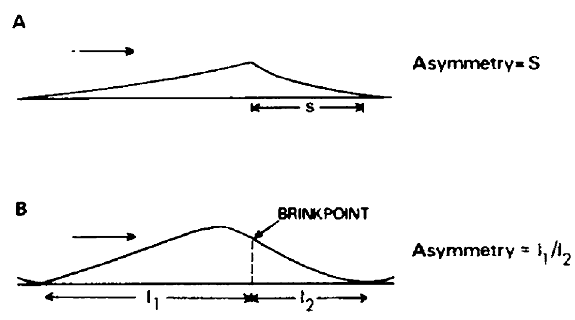 | Figure 1. Ripple asymmetry according to (A) Sharp (1963) and (B) Tanner (1967) |
As per Knighton, 1981, an index of asymmetry should as far as possible fulfill certain basic requirements1. Extreme asymmetry should be expressed by the value ‘1’ and 2. No asymmetry should be expressed by the value ‘0’ The first measure in this paper is the ratio of asymmetry-area (Á) to the total bank-full area of the channel. Á is defined as area between the channel centre line (Lc) and median area line (Lm). Bank-full width (W = wl + wr and wl = wr) of the channel is defined as horizontal length between brink point of levee and high bank. Channel centre line (Lc) is a vertical line from channel bed to W/2 point separating wl and wr and median area line (Lm) is the vertical line from channel bed which divides cross-sectional area of the channel into two equal halves (Figure 2). Width difference (ẃ) is the horizontal distance between Lc and Lm.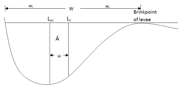 | Figure 2. Definition of parameters of an asymmetrical channel |
How far the channel is skewed to the left or right can be measured by the simple equation 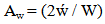 | (1) |
In this measure, if the value is ‘0’, the channel is perfect symmetrical and if it is 1, the channel is 100% asymmetric in nature. Asymmetry in width is not a complete measure of the cross-sectional asymmetry of a river channel because the cross-section is a two dimensional parameter. Therefore area should be incorporated in the index of asymmetry. For the purpose, the asymmetry area (Á) was multiplied with 2 and result was divided by total area (A). Therefore, equation of asymmetry in area can be written as  | (2) |
It seems to be cloned from Knighton’s A* index. Because genetically Aa = (2Á/A) = (Ar-Al) /A. But it is done so that one can calculate ẃ from the cross-section. However, if one directly subtract Al from Ar, it will also give same result because 2Á = Ar-Al.
3. Discussion
3.1. Necessity for Alternative Measure
1. In the index A1, if 2x/w = 0, channel is symmetrical. It is very easy to define the position of dmax in a semicircular and triangular channel. But if the channel is like a perfect rectangle, dmax is everywhere which is very bamboozling. Whereas, the median area line (Lm) is a definite single line for any kind of channel and horizontal asymmetry is brightly determined by the horizontal distance between Lm and Lc.2. Only for a perfect rectangular channel, 2x/w= 0, if dmax and d are single line. 3. For vertical asymmetry or peakedness of the channel, dmax/d ratio was considered. Obviously, greater the ratio more the peakedness but not the ‘vertical asymmetry’.4. Moreover, vertical asymmetry is ignored by the horizontal symmetry. A channel with 2x/w = 0 and leptokurtic nature with ‘vertical asymmetry’ may appear as a symmetric channel producing no vertical asymmetry because product‘0’ (zero) of 2x/w will bring down any value of dmax/d to zero. 5. In 2nd (A1) and 3rd (A2) measure of Knighton (1981), 1st ratio and 2nd ratio of the equations do not give either ‘0’simultaneously (Figs. 3 and Figs. 4). And ‘zero value’ of one part may bring down real numerical value of other part to zero. In the equation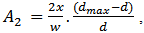 second part
  will never produce ‘0’ (zero) except in a rectangular channel. But by the influence of ‘0’ of horizontal symmetry, any value of second part will be nullified and product of two parts will also be ‘0’.6. To measure the vertical peakedness, real dmax may be compared with ideal dmax The ratio of dmax / d of an ideal cross-section is 2 for triangular channel, 1 for rectangular channel and 1.27 for semicircular channel.
 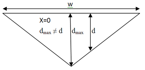 | Figure 3. Symmetrical triangular channel with d≠ dmax |
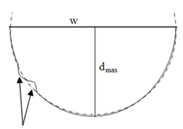 | Figure 4. Symmetrical semicircular channel with d ≠ dmax |
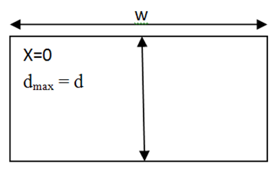 | Figure 5. Symmetrical rectangular channel with d= dmax |
3.2. Empirical Analysis of cross Sectional Asymmetry
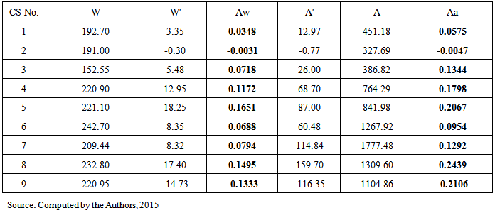
Nine cross-sections of bank-full channel have been drawn based on real ox-bow lake channel (a rejected bend of the River Jalangi in the district of Nadia, West Bengal, Nadia) (Fig.6). Then the two measures have been tested on those cross-sections (Table 1). It has been observed that two cross sections depict negative skewness i.e. CS 2 and 9 are having more linear and areal expansion on the left bank than on the right. But the rest of the channels have the positive skewness i.e. more linear and areal expansion is on the right bank (Table 1). The minimum and the maximum value for the Aw is -0.0031 and 0.1651 respectively while minimum and the maximum value for the Aa is -0.0047 and -0.2106. It is to be observed that minimum value for the both indices (Aw and Aa) has been recorded by the same CS i.e CS No. 2 but maximum value for the two indices have been obtained for the two different CS (Table 1). It proves that there is a positive correlation between these two indices though not perfect. The linear trend value for the indices has derived as 0.911.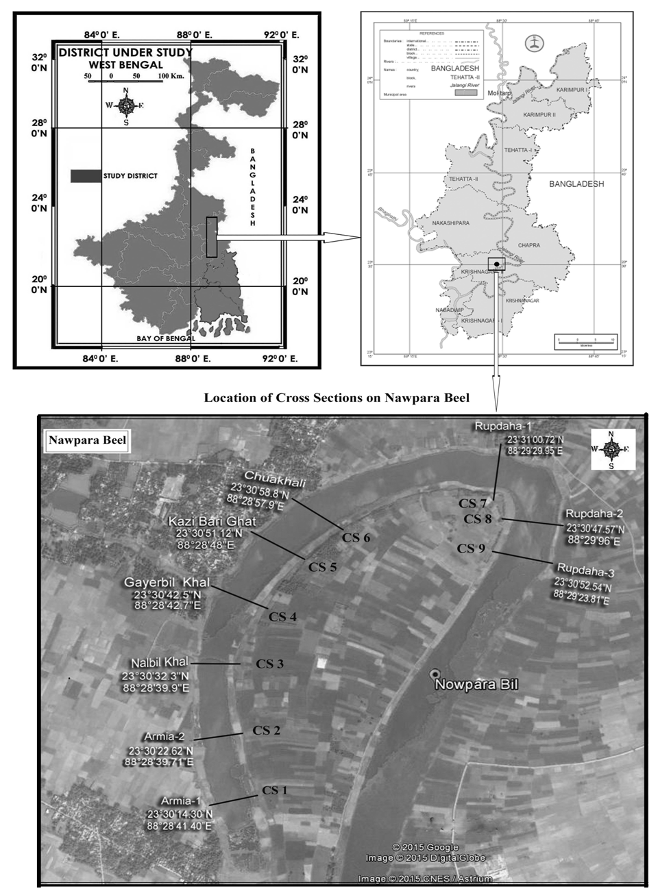 | Figure 6. Location of the Cross Sections on Nawpara Beel, Nadia, West Bengal |
Table 1. Channel Asymmetry indices for Nawpara Beel
 |
| |
|
The values obtained from the Aw and Aa give a definite clustering. For this empirical observation all the values lie within a definite range i.e. between Aa/Aw=1 and Aa/Aw=2. It denotes that Aa will always be greater than 1 and less than 2 of Aw (Fig. 7). 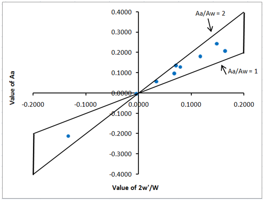 | Figure 7. Relation between Aa and Aw |
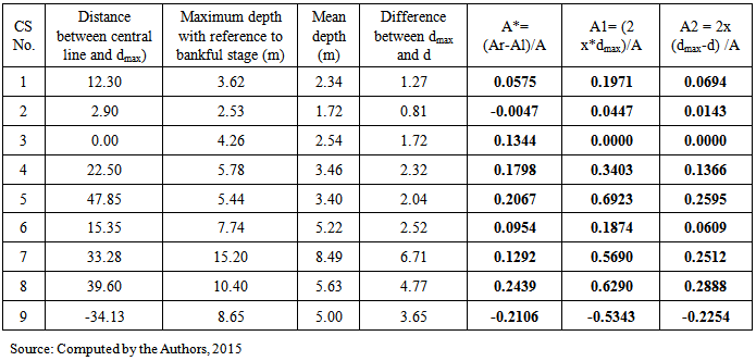
Though the indices proposed in this paper is different in some respects from that of the Knighton (1981), they are associated with each other. This has been analyzed using Principal Component Analysis (PCA). For this analysis four variables (A* or Aa, A1, A2, Aw) and nine CS of Nawpara Beel have been chosen. Variables Aw and Aa have been shown in the table 1 and A*, A1 and A2 in the table 2. As mentioned earlier, A* and Aa are same indices calculated in different approach. That is why in variables four and not five have been taken to avoid repetition of the result.Table 2. Channel Asymmetry Indices of Knighton for the same cross sections of Nawpara Beel
 |
| |
|
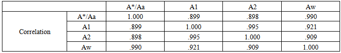
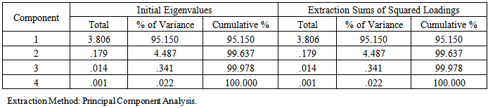
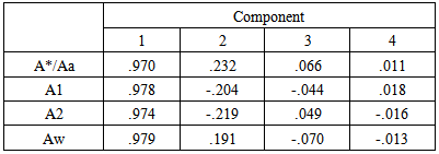
From the multi-variate analysis, it has been observed that all derived values of the correlation coefficient are 0.9 and above i.e each and every indices are correlated strongly with other indices (Table 3). From the eigen value of the PCA, it has been noted that 3.806 (95%) has been explained in the 1st Component, and nearly 0.179 (4.5%) has been explained in the 2nd component. Cumulatively 99.6% has been explained in the 2nd component (Table 4). It definitely establishes the strong correlation between the variables. From the value of component matrix, it can said that the factor loadings for all the four variables are quite high i.e. all are having the value of 0.97 and above and factor loading each and every variables in the 1st component is very close (Table 5). All factor loadings are controlling the system in positive direction as the entire variables have positive loadings in the Component 1. However Aw and A1 have more control over the system in the 1st component. Variables A1 and A2 are controlling the system in negative direction while Aw and Aa in the positive direction (Table 5).Table 3. Correlation Matrix
 |
| |
|
Table 4. Total Variance Explained
 |
| |
|
Table 5. Component Matrix
 |
| |
|
To detect the mutual association between the indices, a 3 dimensional component plot has been prepared (Fig.8). In this plot there are two distinct clustering of indices. Indices Aw and Aa/A* are more closely associated with each other forming a cluster and similarly A1 and A2 are more closely associated with each other forming another cluster. As A1 and A2 are based on the depth consideration, they are quite different from the other indices. 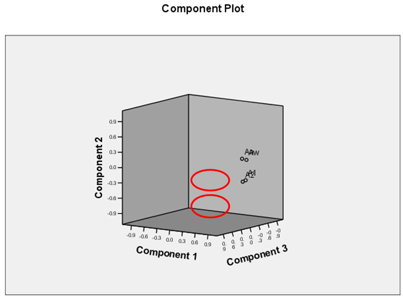 | Figure 8. Component plot of factor loadings for the first three components |
4. Conclusions
Asymmetry of different natural forms and processes has already been quantified and studied by different branches of natural science. Cross-sectional asymmetry of a river channel is a determinant of the alternate ‘scour holes and meandering flow’ of a river (Einstein and Shen 1964; Callander, 1978). But asymmetry in river channel before Knighton (1981) was in the literature (Callander, 1978) only. Therefore his effort is undoubtedly a benchmark to the field. Considering all the aspect of asymmetry indices, it can be concluded that A* is a better index than A1 and A2 to the channel asymmetry where both vertical and horizontal dimensions are incorporated in a single variable of area. Moreover all the pre-condition of an index is maintained in this equation. Measures formulated in this paper are free from some technical problem and anonymity (explained earlier) which are present in Knighton, s indices. Here all kind of symmetrical channel will be expressed as ‘0’ and the extreme asymmetry will never be exceeded by the value ‘1’.
ACKNOLEDGEMENTS
This paper is an outcome of MRP No. F. PSW-097/13-14 dated 18th March, 2014 funded by U.G.C.
References
| [1] | Callander, R. A. (1978). ‘River meandering’, Annual Reuiew of Fluid Mechanics, 10, p-129-158. |
| [2] | Clifton, H. E. (1976). ‘Wave-formed sedimentary structures-a conceptual model’, in Beach and Nearshore Sedimentation, Davis, R. A. and Ethington, R. L. (Eds), Society of Economic Palaeontologists and Mineralogists, Special Publication 24, 126-148. |
| [3] | Einstein, H. A., and Shen, H. W. (1964). ‘A study of meandering in straight alluvial channels’, Journal of Geophysical Research, 69, 5239-5247. |
| [4] | Gour, R. K. and Gupta S. L. Engineering Physics. Delhi: Dhanpat Rai Publications, 1998. |
| [5] | Keller, E. A. (1972). ‘Development of alluvial stream channels: a five-stage model’, Geological Society of America Bulletin, 83, p- 1531-1536. |
| [6] | Kennedy, B. A. (1976). ‘Valley-side slopes and climate’, in Geomorphology and Climare, Derbyshire, E. (Ed.), Chichester, Wiley, pp. 171-202. |
| [7] | Knighton, A. D. (1981), Asymmetry Of River Channel Cross-Sections: Part I. Quantitative Indices’ Earth Surface Processes and Landforms’, Vol. 6,581-588. |
| [8] | Kranck, K. (1972). ‘Tidal current control of sediment distribution in Northumberland Strait, Maritime Provinces’, Journal of Sedimentary Petrology, 42, 596-601. |
| [9] | Leopold, L. B., and Wolman, M. G. (1960). ‘River meanders’, Geological Society of America Bulletin, 71,769-794. |
| [10] | Majumder, T. Rajpat (in Bengali). Kolkata: Ananda, 2011. |
| [11] | Reineck, H-E., and Wunderlich, F. (1968). ‘Zur Unterscheidung von asymmetrischen Oszillationsrippeln und Stromungsrippeln’, Senckenbergiana Lethaea, 49,321-345. |
| [12] | Sharp, R. P. (1963). ‘Wind ripples’, Journal of Geology, 71, 617-636. |
| [13] | Tanner, W. F. (1967). ‘Ripple mark indices and their uses’, Sedimentology, 9, 89-104. |
 Abstract
 Reference
 Full-Text PDF
 Full-text HTML