1. Introduction

Our planet is apparently rich in water but about 97.5 per cent (Hamdy and Lacirignola, 2005) of its water resource is saline and unsuitable for drinking or irrigation or is of little direct use of people; only 2.5 percent is usable but sometimes not readily accessible. About 68.7 per cent of fresh water is piled up in high latitude and altitude as snow and glaciers and 29.9 per cent is remaining as ground water and soil moisture (Anon, 2010). India gets 4000 km³ of water (0.70 per cent of the global or 9.36 per cent of the Asian precipitation) annually as precipitation but it renders home to about 16 percent of world’s population on 2.45 per cent of the terrestrial surface ( NCIWRD, 1999).

The distribution of this natural resource in India is spatially and temporally so uneven that hydrological extremes of flood and drought are annual events in some or other parts of the country. The same is also applicable to West Bengal, a state of India. When Jalpaiguri district received more than 3470 mm of rain, Purulia, Bankura and Birbum on an average receive 1780mm, 1290mm and 1370mm of rainfall respectively in 2013(IMD, 2014). The south-west monsoon virtually generates more than 80 percent of annual precipitation in West Bengal and that pours during the months of June-September. But a single cloud burst over a place can generate more than 60 percent of annual rain within a span of just 48 hours. Likewise to that of India, the management of spatially uneven and temporally skewed rain-water in West Bengal is the most serious challenge for the water-managers.

Water is indispensable for all economic and social development. However, with ever increasing population growth (13.84% in last decade in West Bengal, Rudra, 2013), industrial growth, water pollution and atmospheric changes, the per capita water availability is shrinking day by day (-14.69% in last decade in West Bengal, Rudra, 2013). The Bengal Delta, which was described as areas of ‘excess’ water in the colonial document, now suffers from acute dearth of water during lean months (Rudra, 2013). Increasing water demands vis-à-vis growing water scarcity are expected to reduce diversion of water for agriculture in the future. Efforts are needed to utilize the available limited water resources efficiently. Water resources not only provides water for irrigation but also provide water for a range of other productive uses such as livestock, fishing, home gardens, aquatic products and micro enterprises such as brick making. Hence water is crucial for sustainable development of nation. So, there has been a tremendous pressure on these precious natural resources, mainly due to rapid industrialization and human population. In this direction, works of Roy (2013) and Adhikary (2012) are few to mention.

Keeping in mind, the importance and scarcity of available water resources, it has become imperative to study the behavior of ground water and its fluctuations; model and forecast the fluctuation in advance to help policy formulation for efficient ground water management.

2. Materials and Methods

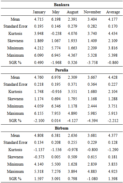
Bankura, Purulia and Birbhum, three districts falling under Red and laterite Zone of West Bengal are characterized by low precipitation. By and large the districts are very dry and most of the portion are belonging to not so developed and under developed zones, millions of people are maintaining their hard lives. Poor or scarcity in availability of long term consistent data on ground water is the main problem in time series analysis on such parameters. The present study has been under taken with the help of ground water level data on seasonal basis (i.e January, May, August and November) for the period 2005 to 2013 in three districts viz. Bankura, Birbhum and Purulia under drier Red and Laterite zone of West Bengal(http://gis2.nic.in/cgwb/Gemsdata.aspx, last accessed on 1/12/2014).

Descriptive statistics are useful to describe the patterns and general behavior of a data set; it includes numerical and graphical statistical measure like minimum, maximum, average, standard error, skewness, kurtosis, simple growth rate.

When dealing with more number of variables in regression analysis, particularly when all the variables are not equally important or efficient in describing the relationships, it becomes difficult to decide on which are the variables to be retained in the multiple regression equation. To know the relationship between ground water level and rain fall pattern, regression analysis along with step down is carried out by taking the ground level data as dependent variable and rain fall (RF₁), lagged rain fall (RF₂), time (t) and three seasonal dummy variables (D₁, D₂ and D₃ for January, May and August respectively) as a independent variable. The multiple regression model can be written as:

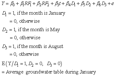Similarly for May and so on, where intercept, are regression coefficient corresponding to independent variables RF₁, RF₂, t, D₁, D₂ and D₃ respectively. In case of dummy variable, if we are interested to know the average ground water level in January, dummy variables for the remaining season will be zero.

For the forecasting purpose use of Box-Jenkins methodology, particularly with time series data, are ample in literaturature; Sahu and Mishra (2013), Mishra et al. (2014) a few to mention. In this paper we have used both simple and seasonal ARIMA to forecast the ground water tables in these three districts. Seasonal data for the period 2005-2012 has been used for building forecast model, while data for the years 2013 are taken for model validation. Box et al. (1994) have generalized the ARIMA model to deal with seasonality and have defined a general multiplicative seasonal ARIMA model, commonly known as seasonal ARIMA model. The seasonal ARIMA model described as ARIMA (p, d, q) X (P, D, Q)_s, where (p, d, q) non-seasonal part of the model and (P, D, Q) seasonal part of the model with a seasonality S, can be written as

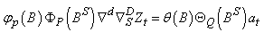where, and are polynomials of order p and q, respectively; and are the polynomials in of degrees P and Q respectively; p=order of non-seasonal autoregressive operator; d= number of regular differencing; q=order of the non-seasonal moving average; P = order of seasonal auto-regression; Q=order of seasonal moving average. The ordinary and seasonal difference components are designated by and 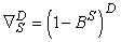of orders d and D; B is the backward shift operator; d is the number of regular differences; D is the number of seasonal difference; S = seasonality. denotes observed value at time t, where t = 1, 2, . . . . . 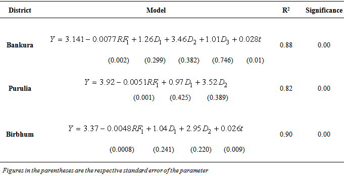k; and is the Gaussian white noise or estimated residual at time t.

Given a set of time series data, one can calculate the mean, variance, autocorrelation function (ACF) and partial autocorrelation function (PACF). The calculation enables one to look at the estimated ACF and PACF which gives an idea about the correlation between observations, indicating the sub-group of models to be entertained. This process is done by looking at the cut-offs in the ACF and PACF. At the identification stage, one would try to match the estimated ACF and PACF with the theoretical ACF and PACF as a guide for tentative model selection, but the final decision is made once the model is estimated and diagnosed.

Among the competitive models, best models are selected based on minimum value of Akaike Information Criterion (AIC), Bayesian Information Criterion (BIC), Mean Error (ME), Root Mean Square Error (RMSE), Mean Absolute Error (MAE), Mean Percentage Error (MPE), Mean Absolute Percentage Error (MAPE) and maximum value of R² and of course the significance of the coefficients of the models. Best fitted models are put under diagnostic checks through auto correlation function (ACF) and partial autocorrelation function (PACF) of the residual.

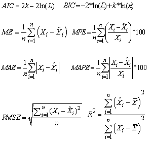
are the value of the i^th observation, mean and estimated value of the i^th observation of the variable X and k is the number of parameters in the statistical model, and L is the maximized value of the likelihood function for the estimated model.

3. Results and Discussion

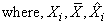
The ground water level in the selected districts seem to be depleting in May month which may be due removal of water for irrigation purpose, more water absorption by plants particularly deep rooted plants and other water evolved activates. Since 2006, among the selected districts, on an average Purulia is found to be more fluctuating district with a standard error of 0.277 meter (Table. 1). Within the districts, ground water level shows more variation in August, November, November with a standard error value of 0.371, 0.229, 0.282 meters respectively in case of Purulia, Birbum and Bankura. Purulia and Bankura districts show the negative growth rates of -2.21 and -0.86 percent respectively. Thereby indicating the decrease in ground water tables which may be due to implementation of ground water recycling/recharging programs like constructions of water cannels, rain water harvesting techniques, improved irrigation methods in recent years.

Table 1. Perse description of ground water table in Bankura, Purulia and Birbhum

The result of stepwise regression is framed in table. 2. The results indicates that in all the three districts ground water level improved significantly as rainfall increases in the respective month. But the significant positive coefficient for remaining all the independent variable indicates that the ground water level is depleting years to come. These regression equation provide the average ground water level for different seasons under given rainfall condition.

Table 2. Step wise regression model

From the results of SARIMA modeling (Table.3), one can find that none of the series is seasonally stationary in nature; first order seasonal differencing is necessary for all the series to make these stationary. The fitted model ranges from ARIMA (0,0,0)(0,1,0)₄ to ARIMA (3,1,3)(3,1,3)₄. Among the competitive models which satisfies the maximum criteria (higher R², lowest AIC, BIC, ME, RMSE, MAE, MAPE and MPE) and having significant parameters are retained for further use. The model ARIMA(1,0,0)X(1,1,1)₄, ARIMA (2,0,0) (1,1,1) and ARIMA(1,0,1)(2,1,0) are found best suited for Bankura, Purulia and Birbhum respectively.

Table 3. Best fitted SARIMA models

These models are again validated not only by comparing observed and predicted values for the 2013 (four season, Table.4), Figure. 2 shows that observed values are closely matching with those of the expected values during the period of validation. Now, the above best fitted models are used to get the forecasting values for 2014 (four seasons) and same is presented in table. 4. It can be seen from the table that for Bankura and Purulia the selected SARIMA models have tendency of over estimating while for Birbhum it has got tendency of underestimating. What is alarming from predicted values for 2014 is that in both the districts of Bankur and Purulia ground water table will mostly go further downwards in majority of the seasons while in Birbhum this may improve a bit in all the seasons. Using the above estimated values for ground water levels in these three districts ground water management strategies could be framed for the 2015.

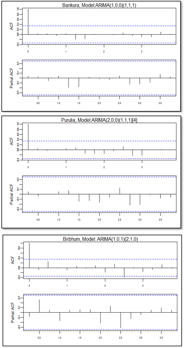Figure 1. Residual ACF and PACF graphs

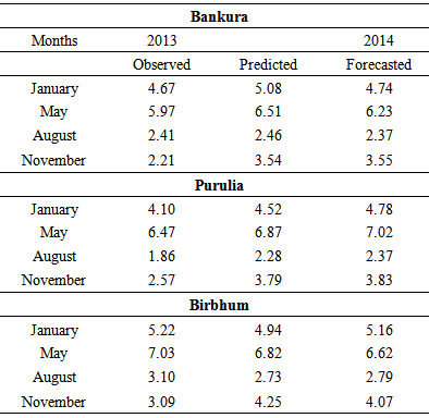
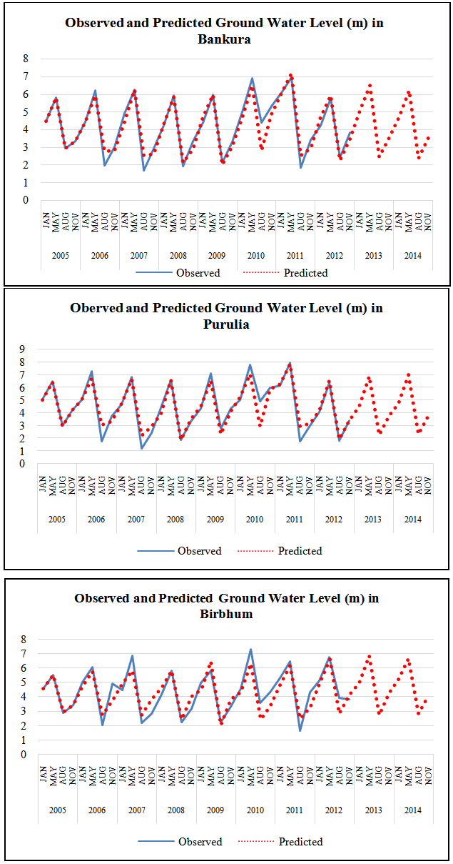Figure 2. Observed and forecasted value

Table 4. Model validation and forecasting values of ground water level in meters

4. Conclusions

From the study one can find contrasting features in groundwater table depth. While the average value for ground water table shows negative growth rates for Purulia and Bankua but positive for Birbhum district; inter season differences are also there among the districts. Fluctuations in the depths of ground water table can very well be explained with linear multiple regression equation using dummy variables for different seasons. Like other examples, the SARIMA models can very well be explored for modeling and forecasting ground water table in different places. Forecast values shows somewhat different picture than the average behavior of the series. Forecasting value shows that groundwater depth in Birbhum will reduce but for other two districts, this will increase. Thus there is a need for formulation of plans and its execution to arrest the growth in groundwater table depths in Purulia and Bankura.