1. Introduction

Of the three general state of matter, the liquid is most complex. It has neither the extreme order of the solid nor there extreme disorder of the gaseous state. The liquid state remains the one which is least understood and most difficulty to model in a satisfactory manner. The liquid, most difficult of all to model is our commonest one, water. A model is a difficult task still is to be developed to account for all types of aqueous solutions. A vast number of research articles have been devoted to the structure of water and aqueous solution. it will be an impossible task to mention even a small fraction of these [1, 2]. However, a central work landmark in this respect was the fundamental work of Bernal and Flower [3] followed by Feank [4] –water contains ‘cluster’ of hydrogen bond molecules, code name ‘iceberg’. Nemethy and Schrage [5] structure is temporary and chaining ‘flickering cluster’. Ben-Naim [6] –there is a dynamic equilibrium between some bonded and non-bonded water molecules, with hydrophobic interactions between solute particles being important. Bernal [7] also favored continuum theories rather than mixture theories of water structure based on the concept of strain and bent hydrogen bonds.

Following a critical survey of the vast recent literature Schmid [8] stated that nature of liquid water can be understood in terms of a competition between H-bond (coulomb) and dispersion (van der Waals) forces. Since the bonding characteristics in crystalline face carry over to the liquid state, any molecular dynamics model of the liquid would have first to reproduce well the ice polymorph structures under appropriate thermodynamic condition.

Once it has been recognized that water is a structure liquid, the immediate question that arises is how this structure changes when we add various solutes in water. These are, of course, a different meaning, view and definition of the concept of the structure of water [9, 10].

Solubility is an old subject, although most of the early interest was in the solubility of solids in water, which is still an important area of research and applications. Early quantitative measurements of the solubility of gases, a more difficult measurement were made by William Henry, as well as by Cavendish, Priestley and others. Henry studied the pressure and temperature dependency of air, hydrogen, nitrogen, oxygen and other gases in water. He discovered, among other things that oxygen is more soluble than nitrogen in water. This is an early example of the principle that is the basis of preferential extraction of one gas from a mixture of gases by use of the solvent.

For calculating the solubility of gases in water, Swope and Andersen [11] developed a coupling parameter method for calculating the chemical potential of a solute in a solution using molecular dynamics calculations and applied it to the study of inert gases in water. The calculation used a modified version of the revised central force model for the water-water interaction and a Lennard –Jones interaction between the solute atom and the oxygen atom of water molecule. The revised central force model and it’s modification given by Swope and Andersen is not a perfect model of water. In addition, they omit the long ranged dipole-dipole interactions. The real repulsive interactions are presumable also dependent on the orientation of water molecule and not just the distance of the atom from oxygen.

The statistical mechanical theory of fluids employing distance scaling as a coupling procedure and hence called scaled particle theory (SPT) has been developed by Reiss et al [12-14]. Pieroitti [15] developed a theory using the SPT for prediction the solubility of gases in water. The most surprising aspect of the theory is that it appears to predict the thermodynamic properties (Gibbs free energy, entropies, enthalpies, molar heat capacities etc) of gases dissolve in water successfully. The abnormal thermodynamic properties of aqueous solution are discussed in light of the enthalpy and entropy of cavity formation. Basic to the theory is the use of term derived by Reiss et al for the calculation of reversible work of making a cavity in a hard sphere solvent. The prescription used for the gas dissolution process in water is a very simple one. The gas solute is discharged to a hard sphere, as a hard sphere makes a cavity in the real solvent. Finally the solute is recharged and allowed to interact with solvent molecule. Pieroitti assumes equivalency of this of this reversible work required for cavity formation and cavity formation energy (CFE). Pierotti [16] compare to reversible work require producing cavity in a fluid and the same require for macroscopic cavity formation in classical thermodynamics. This comparative calculation can be avoided as Matyushov and Ladanyi [17] they directly calculated the cavity formation energy from the exact geothermal relation valid for sphere fluid. In the present communication this cavity formation energy expression is used to calculate the solubility of gases in water.

2. Methodology

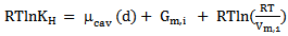
The equation of solubility

The Henry’s law constant (solubility) and thermodynamic functions of solution pertaining to the solution process calculated in usual manner utilizing scale particle theory (SPT) formalism, considering dissolution of gas in a liquid takes place through two steps:

a) First, the creation of a cavity in the solvent of suitable size to accommodate the solute molecules, its diameter exactly the hard sphere diameter of the solute gas. This is referred to as a cavity formation process. The free energy associate with this process is called cavity formation energy (CFE /βμ_cav).

b) The second step involved introduction of solute molecule in to the cavity of the solvent and hence interaction between solute and solvent occurs according to some potential law. The energy a associated with this process is called Gibbs free energy of interaction.

The solubility of gas in liquid is described by Henry's law constant (K_H) as

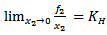(1)

Where f₂ is the fugacity (essentially pressure) of the gases and x₂ is the mole fraction of solute in solution.

For extremely dilute solution, from statistical mechanics Henry's law constant can be written as

(2)

where μ_cav(d) is the cavity formation energy to make one mole of cavity in the solvent water and each cavity is sufficiently large to hold one gas molecule. G_m.i is the molar Gibb’s free energy of interaction between the solute in the cavity and the surrounding molecules of water, R is the gas constant T is the system temperature and K_H is Henry’s law constant of gases in water and V_m,1 is the molar volume of the water.

Computation of Cavity formation energy of water

The expression of cavity formation energy that discussed in previous paper by Guha and Panda [18-22], and Matyushov and Ladanyi [17] was extended to solubility of methyl fluoride, methyl chloride, carbon monoxide and nitric oxide and nitrous oxide in water solvent as

(3)

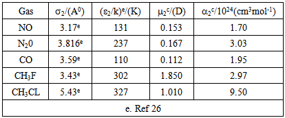
where is the "compactness factor" of solvent. The number density of solvent is define by ρ = N_A/V_m,1, N_A is a Avogadro’s number and V_m,1 = density/molecular weight, σ₁ hard sphere diameter of the solvent and d = σ₂/σ₁, σ₂ is hard sphere diameter of the solute gases. The last term of the above equation is related to hydrostatic pressure for gas solubility in incompressible liquids at 1 atmosphere pressure, it can be neglected.

Computation of Interaction energy of solute with mixed solvents

This term represent the partial molar free energy of interaction when a solute molecule introduce into a solvent cavity. This consists of three terms; a dispersion energy term, an inductive energy terms and dipole-dipole interaction energy term.

Solubility of polar gases in water was calculated by following expression

(4)

where the mixing potential parameters ε₁₂ and σ₁₂ are related to the pure component parameters by approximate mixing rules and

where ε₁ and ε₂ are Lennard-Jones (6-12) parameter for solvent solute gas respectively and μ₁is the dipole moment of the solvent.

3. Results and Discussion

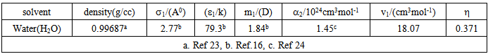
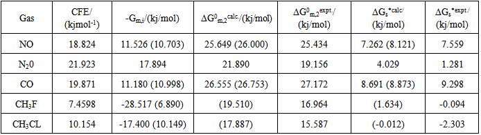
The cavity formation energy of water is calculated by means of equation (3) at 298.15K given in the table1. The cavity formation energy plotted against ratio of hard sphere diameter of solute (gas) to water which shown in Figure 1. The necessary physical parameters of water are given in the table 2. From this curve we see that the cavity formation energy increases monotonically with rise of ratio of hard sphere diameter of solute gases to water. Since latter decreases with decrease of hard sphere diameter of solute gases, so we concludes that water easily form cavity when a small solute molecule across it than larger one.

Table 1. The cavity formation energies (CFEor βμcav) of water at temperature 298.15K and 1 atm. pressure

Table 2. Selected physical parameters of liquid water at temperature 298.15K

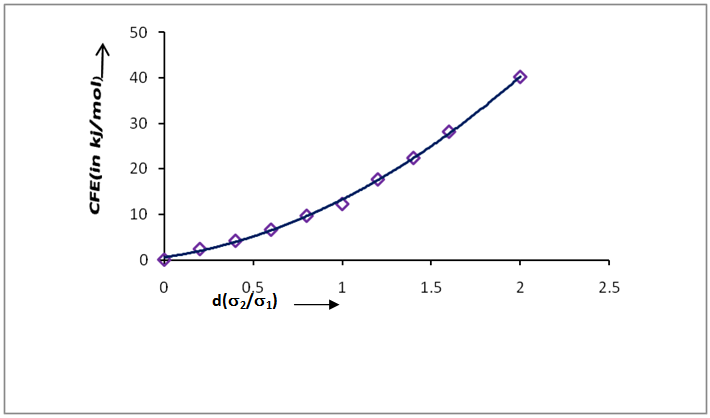Figure 1. Cavity formation energy, CFE(kj/mol) of water with ratio of hard sphere diameter at 298.15k

The Henry’s law constant for polar gases such as methyl fluoride(CH₃F), methyl chloride(CH₃Cl), nitrous oxide(N₂O), nitric oxide(NO) and carbon monoxide(CO) are calculated by means of equation(4). Table 3 contains calculated and experiential lnK_H. The values within first backed is the results considered above molecule behave as non polar. Require molecular parameter for polar gases is given in table 4.

Table 3. Solubilities in terms of Henry’s law constant some polar gases dissolved in water at temperature, T=298.15K and pressure p2=1 atm

Table 4. Selected physical polar gases

Molar Gibbs free energy of polar and non-polar gases in water at 298.15K

The standard Molar Gibbs free energies of solution process both theoretical and experimental for methylfluoride (CH₃F), methyl chloride (CH₃Cl), nitrous oxide(N₂O), nitric oxide(NO) and carbon monoxide(CO) gases in water appear in Table 5. They were calculated from solubility results using the following relation.

Table 5. Cavity formation energies, interaction energies, Gibbs free energies of solution and Ben-Naim thermodynamic quantities of polar gases in water at 298.15K

ΔG⁰_m,2 = RT1nK_H given by Clever and Battino [27] for the hypothetical solution process

M(gas, hyp. 1 atm pr)à M(soln., hyp, x₂)

where ΔG⁰_m,2 is the molar Gibbs free energy transfer from vapor phase at temperature 298.15K and 1 atmosphere pressure. For gases such as methyl fluoride and methyl chloride experimental values more than a factor of 1. In all fairness to the theory, this implies that it does much better in predicting the Gibbs free energy change associated with the solution process.

Ben-Naim thermodynamically quantity, ΔGs* for aqueous solution

Ben-Naim [28] has warned against using the hypothetical standard state, particularly when the goal is to derive salvation properties from arguments of statistical mechanics. Hence, it is preferable to introduce the Gibbs energy of salvation on the density number scale.

ΔG_s*=ΔG⁰_m,2-RT1n(RT/V_m,1)=G_m,c+G_m,i where RTln (RT/V_m,1) is a term to correlate ΔG_s* with the standard state bases on mole fraction. From above relations it is clear that ΔG⁰_m,2 take into pure solvent properties whereas ΔGs* express directly the interaction of the solute. We will see later that these differences have importance consequences. The experimental values of ΔGs* for polar gases in water were given in the Table 5. For all the gases, methyl fluoride and methyl chloride the salvation process is not favored thermodynamically under Ben-Naim considerations as ΔG_s*> 0. This indicates that a prevalence of cavity term (positive) and (negative). This explains the low solubility gases consider here in water at 298.15K temperature and 1 atmosphere pressure. For methyl fluoride and methyl chloride ΔG_s*< 0. So, dissolution process in water for these gases is favored thermodynamically under Ben-Naim consideration. Hence, mole fraction, methyl fluoride and methyl chloride are relatively large or lnK_H are low than other gases consider there.

4. Conclusions

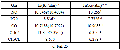
There is some discrepancy between calculated experimental Henry’s law constant. But the discrepancy for polar gases especially methyl fluoride and methyl chloride are very large. The results in Table 4 within the first backed that if these solutes are consider non-polar(only dispersion force contribution to interaction energy) then calculated and experimental logarithm of Henry’s law constant will be closed to each other. It is as if the collective effect of solvent electric field on the solute particle. In, addition lnK_H in water depends upon two factors: one is cavity formation energy and other is interaction energy. The calculated cavity term extremely sensitive to the choice of the diameter of the water since hard sphere diameter of solvent water (σ₁) is raised to the sixth power in the calculations.

The value of hard sphere diameter of solvent and solute available in the literature may be calculated from the surface tension viscosity, second virial coefficient, heat of vaporization, molecular dynamic simulation and gas solubility etc. The results obtained from different experiment are not unique. As example hard sphere diameter in ⁰A of water are 2.77(ref16), 2.76, 2.75(ref 15) 2.86(ref 29) 2.89(ref 30) 2.56 and 2.922 ref(31) 2.65(ref 32) so exact choice of this parameter is difficult and it is possible that values used were in error. The differences between experimental and calculated values arise from this choice. Moreover the solute and solvent interaction energy is sensitive to the values of ε/k the Lennard-Jones parameter of the solute and solvent. The value of this parameter is not also unique as for example argon ε/k range from 117 to 125. So proper choice of ε/k and σ gibes the exact experimental result s as expected.

In conclusion we can say that however, present statistical mechanical approach, in spite of the rigid hard sphere model employed, is able to reproduce rather successfully to predict solubility of gases in water. If we could choose proper value of molecular parameters then it can give exact experimental results as expected.