1. Introduction

Credit risk is one of the most important kinds of risk in banking sector. Particularly, the relationship between business cycle and banks’ loan losses was one of the hot debates in recent economic literature especially in relation to financial stability analysis. The quality of loans can be one of the factors that limit the banks' loan supply and effect on investment spending. Although banks have a significant role in transmission of monetary policy, in the meantime their performance is strongly influenced by monetary and fiscal policies. Thus, a sensitivity analysis of the credit risk of the loan portfolio is in great importance[23]. The financial crisis in recent decades and their considerable costs to the real economy and financial institutions have highlighted the importance of this position. Malaysia is among the countries where the banking system was affected by the financial crisis of 1997. Following the crisis, many banks have failed and the Malaysian government was incurring considerable costs to revive the banking sector.

According to some studies such as[35] the most important reason of this crisis was the lack of enough supervisory and regulatory rules in banking system beside noticeable increase in foreign private capital inflow (short-time debts). However, given the relative stability of the banking system created in recent years, another form of competition between the banks providing credit to households and small businesses has been created. By growing share of bank loans in these sections, banks are exposed to the risks of shocks on macroeconomic variables. Macroeconomic variables can effect in/directly on banks loans quality and their transitional role. Thus policy makers and bankers are always concerned with the financial stability and looking for tools to better manage banks’ credit risk. One of the risk indicators that are used in literature of banks’ credit risk is Non-Performing Loans (NPL). Hence the main objective of this study is to analyze relationship between banks loans quality and macroeconomic variables by using a dynamic panel data model in Malaysian commercial banking system for the period of1997-2012. The result of this study can be helpful to bank supervisory and economists to adjust banking system stability and economic policies.

2. Theoretical Background and literature

In recent years, the studies of the credit qualities pay more attention to the influence of macroeconomic variables and have found same empirical results. The earlier studies about standard credit risk models have been done by[16],[18],[21] and[27-29]. They follow each other’s' studies in this area and at least[32-33] constructed a model that include the macroeconomic variables such as GDP, interest rate, government expenditure, housing price index and etc. that influence a firm’s probability of default. He used a pooled logit regression and confirmed more relationship between macroeconomics factors and the Probability of Default. After this study many different surveys have used macro stress test approach to explain the behavior of banking systems against adverse macroeconomic shocks.

In order to assess different features for banks’ loans in different situation, most of the studies done bank-level data, have used bottom-up approach and applied panel data methods to investigate banks’ credit behavior (See[11], [13-15],[30] and[34]). Since in these researches, Non-Performing Loan ratio is used as a risk indicator; so it is tried to gather a summary of the literature, focusing on studies that examine the macroeconomics determinants of this variable in banking system.

A group of studies have investigated the effects of macroeconomic variables on NPLs changing (See[12],[17] and[26]). They have shown that bank specific factors have important roles in NPLs future behaviors. According to a panel data study on some countries in Europe by[25], the monetary policies, unemployment and income impact effectively on NPLs. In other different studies on Nordik by[6] and Austrian banks by[9], a significant relationship between loan quality and some macroeconomics variables such as unemployment, interest rate and business cycles is indicated. By a panel data model in Greek banking system,[20] shows significant connection between NPLs changes and macroeconomic variables especially interest rate, GPD, public dept and unemployment. They categorize loans in three groups including consumers, business and mortgages. Reference[31] by means of a panel data model and dividing the bank loans to 21 granular parts investigate the effects of GDP growth with different quarterly lags on LNPs for Brazilian banks.

Some researches focus on explanation of bank specific effects on NPLs such as[7],[10],[19] and[22]. Results from these studies indicate that efficiency indexes from different aspects such as management, skimming, cost and moral hazard can affect the NPLs. After recent financial crisis many studies try to depict linkage between the debt crisis and banking fragility such as[24].

Few studies have been conducted on credit risk in Malaysian banking system. Refrence[1] find some key determinants of credit risk of commercial banks in emerging economy (including Malaysia). They use a combination of three theory including capital asset pricing, Hamada’s risk and leverage theory and Markowitz’s Portfolio theory to create a theoretical relationship between credit risk and eight bank specific factors. NPL implied as a credit risk factor and their main result is that, credit risk in emerging countries related to several bank specific factors. Also[2] indicate a significant negative relationship between credit risk and GDP in OECD and Asian countries. According to new structure of banking system and sensitivity of household and SMEs sectors as important part of their credit customers, to macroeconomic shocks it requires more attention to investigate the effects of macro variables on credit risk.

3. NPL and Macroeconomic Variables in Malaysia

According to the literature, there is not a standard framework to analyze effective factors influencing loans quality. Following the models on the studies mentioned above, in this paper some important macroeconomic variables are selected as factors affecting credit risk including: GDP growth (GDG), lending interest rates (LR), Consumer Price Index (CPI) or Inflation, foreign direct investment outflow as a percentage of GDP (FDua) and Domestic total Credit growth (DCg). Also following the literature, Non-Performing Loans to total loans ratio (after this it is said NPL) is used as a proxy for loan quality or credit risk; because borrower’s ability to repay debt in boom and recession will be affected by the NPL in banking system. The bank balance sheet data set (loans, assets and NPLs) have been collected from Bank Scope data base from 1997 to 2011. And data for macroeconomic variables are collected from World Bank's data bank. As there is not homogeneity between the banks based on the date of establishment, so our data is not balanced and is taken from 23 Malaysian commercial banks with 252 observations.

A look at the banks' loans shows that credit quality is extremely heterogeneous based on different size of banks. Comparing the banks’ average of NPL and their standard deviation in figure (1) shows this feature. In this figure the banks’ code numbers are sorted based on asset size from big to small size. This figure shows that the banks with small size have more NPL in average and more standard deviation. The trend of NPL and macroeconomic variables are comparable in figures (2 and 3). According to figure (2), the negative association between output growth and also lending interest rate with NPL is quite evident. But the exact relationship among these variables with an interval necessarily needs to implement econometric model. As it is shown in figure (3), there is a positive connection between NPL and loan growth. After 1997 crisis rapid credit growth and the supportive economic environment led to increase of NPL until 2004 with a series of pulses. After 2004 banking system faced a relative stability and NPL despite the increase of loans, had a decreasing trend. This feature continued until 2008 and the negative impact of the global financial crisis on the macroeconomic (decrease in economic growth) and financial environment led to stop NPL downward trend. This figure also shows an inverse relationship between FDau and NPL but linking with an interruption between them is controversial which can be discussed based on econometric model’s results.

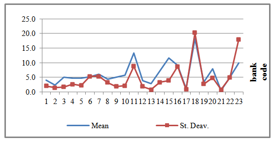Figure (1). Selected statistics of NPLs across 23 banks 1997–2011 in percentage

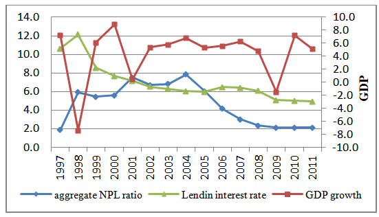Figure (2). NPL in total bank system in comparison with GDP growth and lending rate in Malaysia

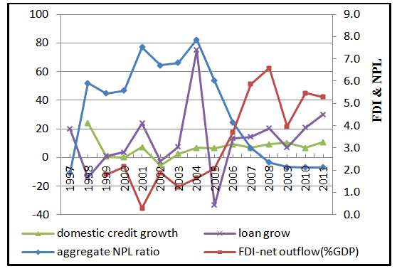Figure (3). NPL in total bank system in comparison with total domestic credit growth, FDI-net outflow and total loans growth in commercial banks

4. Econometrics Model

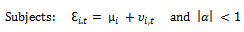
An econometric model is used to explain the behavior of banks’ loan quality and identify factors affecting its changes. To this end, the ratio of net Non-Performing Loans to total loans (NPL) is used as indicator of loan quality or credit risk. Following the empirical studies on NPL based on dynamic panel data models, in this study also a dynamic framework is designed to survey the NPL behavior in Malaysian banking system. Since some of the banks have less information so the Dynamic Model Panel Data will be better to analyzes the sensitivity of NPL to macroeconomics factors. The sample is unbalanced because of the exit or merge of some banks and the incorporation of new ones. Based on a general dynamic panel data model the main equation in this study is:

(1)

that subscripts of t and i show the time dimension and cross sectional of the panel. The bank specific unobserved effect is shown with is the error term. Β is the k×1 vector of coefficients for explanatory variables (X that is a k×1 vector). In this paper according to literature the GDP growth (GDG), total domestic credit growth (DCg), net outflow of foreign direct investment (FDau), consumer price index (CPI) and the lending interest rate (Lr) considered as the most important factors affecting on NPL. Also these factors are used with two years lag in the model. In this regard, it is noteworthy that data limitations prevented the use of variables that delayed for more than two years.

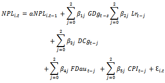
(2)

The coefficient is expected to be positive but less than one, and coefficients are expected to be negative and reflect deteriorating loan quality during the economic downturn. if j=0 have to be positive because when interest rate increases the debtors cannot borrow more to improve their financial situation and solvency. At the same time demand for new funds for new projects is reduced; so in the next few years NPL is likely to be reduced. Hence it is expected that when j>0 to be negative. The increase in loans by commercial banks typically have a positive impact on NPL but the increase of the total domestic credits will have a positive impact on reducing the NPL so that is expected to be negative. When j=0, is expected to be positive because outflow of foreign funds lead to financial limitation for domestic investors. Based on empirical results the can be negative or positive depending on the economic condition. If inflation leads to increase the value of costumers’ assets, consequently the will be negative.

5. Estimation Methods

The inclusion of the lagged dependent variables in banks non performed loan function means that there is correlation between lag of independent variable and the error term which include bank-specific effect and the is endogenous. Therefore, the dynamic panel data estimation with Ordinary Less Square (OLS) and Fixed Effects methods (FE) will be bias. If the sample be large this problem will be solved but in small samples it needs to use the methods that reduce this bias. Reference[3] suggests GMM estimators to solve the endogeneity problem. To this end the firm specific effecthave to be removed from the equation (1). Reference[3] shows that by using first difference method the firm specific effect can be eliminated but a new kind of bias is introduced by means of the correlation between the transformed lagged dependent variable and the transformed error terms by first deference. Also if some of the explanatory variables be predetermined it means that there is correlation between error terms and explanatory variable or = 0 for s < t but ≠ 0 for s ≥ t.

To solve this problem[4] suggests using the untransformed regressors or lagged level as instrument for the transformed variables (First differenced GMM method). On the other hand according to[8], if the lagged dependent variables are persistent during the time or tend to be random walk, so lagged levels of these variables will be weak instruments in first difference equation of regression. Therefore, a system GMM approach is suggested by[8] to avoid the probabilistic bias with the differenced estimator. In this proposed regression in differences and regression in levels are combined and the instruments for independent variables in levels are the lagged differences of the corresponding instruments.

Notably,[3] suggests two different One-step and two-step methods to estimate of GMM and System GMM models. In one step method it is assumed that the error terms are independent and homoskedastic between units. But in two steps the error terms extracted from first step are used to create a consistent estimate of the variance–covariance matrix in order to relaxing the assumption of independence and homoskedasticity of error terms; because on this condition the result will be different.

6. Estimate Results

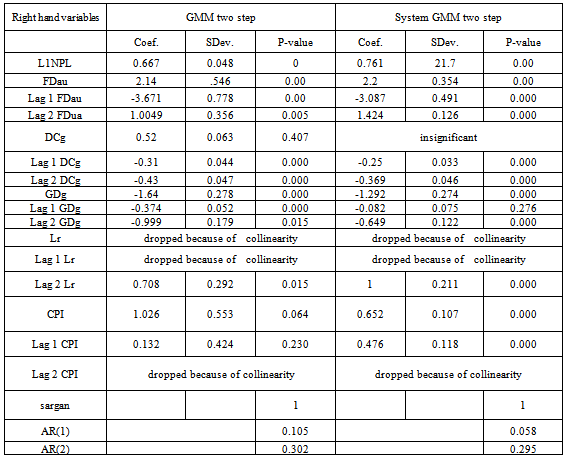
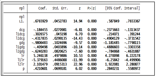
To achieve better results and interpretation, different methods have been used to estimate the coefficients and all the models were computed over the entire sample of banks. First of all the GMM and system GMM model estimated with one step method but most of coefficients are not significant. Also the Sargan test show that over identifying condition about combination of instrument variables is not correctly specified. Hence the two step method is used in both GMM and system GMM model. The results of these two models are indicated in table (1).

Table (1). Summary results of exploratory panel regressions

As it is shown, the Sargan test in both models indicates the optimal combination of instrumental variables used in the estimation of the models. Also the autocorrelation test results suggest there is no autocorrelation between error terms. The results of the exploratory regressions are in line with expectations and extremely robust under alternative estimation methods. The coefficient of the lagged dependent variable is 0.66 and 0.76 in GMM and System GMM models respectively. It means NPL is persistence. Since the System GMM model used the comprehensive instrument variables and the correlation between explanatory variables and error term is tested and solved this potential problem; therefore, the results based on System GMM model is used to interpret the coefficients.

As it is shown in the table (1), both of GDP growth and domestic credit growth have negative effects and both lending rate and inflation have positive effects on NPL ratio. The share of FDI-net outflow from GDP has positive effects on NPL ratio in level due to reduced access to financial resources by domestic investors to pay their debts. But after one year it leads to decrease NPL. It means that outflow of foreign investments leads to less domestic investment and consequently less NPL in the future. If the percentage of FDI outflows from GDP, increase 1unit (for example if it shifts from 4% to 5%) NPL ratio in commercial banks will increase 2.2 units (for example it will shift from 2% to 4.2%) but the next year it will decrease 3 units. GDP growth has negative effects on NPL ratio under any circumstances and its contemporaneous effect is more than one-and two-year interval effects. According to the results, one unit increase in GDP growth leads to 1.3 units decrease in NPL ratio simultaneously and 0.6 units after two years.

About the growth of lending by commercial banks it is noteworthy that the effect of this variable was significant, but its amount is very small; therefore, the growth rate of total domestic credit to private sector (DCg) was used as an alternative variable. The estimated results show that any increase in DCg with two year delay has a positive effect on NP. It is noteworthy that the DCg in level was dropped because of collinearity. Also the Level and one-year lag variables of lending rate (Lr) have been removed for the same reason. But this factor has important role in banks’ operation and loans quality. Based on the correlation matrix of explanatory variables, the lending interest rate is strongly correlated with FDI-net outflow in percentage of GDP (FDau). Thus the model was re-estimated by replacement of FDau with lending interest rate and its intervals. The results of this model are shown in table (2). As it is indicated the lending interest rate has strongly contemporaneous and positive effect on NPL and after one year it caused a decrease in it. When the interest rate grows at short time, access to new funds to replace existing debt will be lower and consequently the NPL will increase. On the other hand demand for loans by new customers will be decreased and over the coming year the NPL gradually will be less. As a result, one unit increase in lending rate leads to 5 units increase in the NLP and after one year it exactly as the negative effects.

Table (2)

It is worth mentioning that most of different estimated models, the coefficients of one and two-year lag price were not significant and the price level variable has had a positive impact on NPL.

7. Conclusions

The econometric estimation results show that there is a strong evidence of the cyclical sensitivity of loan quality in Malaysia’s commercial banking system. Based on the results, lending interest rate and FDI-net outflow (%GDP) are the most effective factors on NPL ratio with simultaneous positive effects and a reverse effect with one-year delay. This situation is an evidence of the extreme sensitivity of the commercial banking system in Malaysia as open economy to FDI. Also there is a robust negative relationship between NPL and GDP growth with the effects operating with up to two year lags. Inflation and domestic credit growth have positive and negative effects respectively and their effects last for up to two years, but a mild.

So it can be said that the impact of external shocks on the domestic banking system is more than internal shocks. Meanwhile, the effects of monetary policy shocks are greater than demand and supply shocks. These results can influence decisions and policy outcomes by economists; it also affects the prediction effects of monetary and fiscal policies and above all to combat the negative effects of external shocks. On the other hand, banks can forecast the effects of economics shocks on their loans’ quality and start implementing actions required to adjust their capital adequacy to deal with potential risks.

Also these results can be merged with vector autoregressive (VAR) model that extracts the relationship between some macroeconomics variables systematically. This model is very useful to illustrate the impact of shocks and can be used in estimation an out-of- sample simulation of NLP for banking system under different scenarios.

Notes

1. Initially the Loan growth for each bank as a bank specific variables insert to the model but its coefficient was always insignificant. Hence the domestic total credit to privet sector selected as alternative variable.

2. It means that the NPL cannot be non-stationary series

3. OLS estimator will be bias upwards because of correlation between error terms and lag depended variable. And Fixed Effects estimator will be bias downward because in this method that contains the effects of the variables which are constant over time but vary among units, is removed from the model.

4. If this coefficient equal to 1 it means that the depended variable (NPL) is not stationary and in this situation it is necessary to used first difference GMM model. It means that we have to use first difference of NPL as depended variables.